How To Use QUERY Function In Google Sheets

QUERY function in Google Sheets is probably the most powerful and useful function you can use to manipulate data and analyze it according to your preferences in an Excel file or a Google Drive file. The function allows people to use database-type commands in Google Sheets, which makes it a crucial formula for data analysis in data science.

You can search and filter data in a data set in any way you want using the QUERY function. The Google Sheets query function is an uphill task to master, especially if you are a beginner. The format of a typical QUERY function is similar to SQL and brings the power of database searches to Google Sheets.

How To Use Query Function In Google Sheets

It is essential for users to know that you need to practice the QUERY function in Google Sheets to master it. Let’s have a look at this formula in detail and see how it can be used in different scenarios.

Now, let’s take a look at these steps in detail with images after studying the function syntax.

QUERY Function Syntax

The Syntax of the QUERY function in Google Sheets is as given below.

=QUERY(data, query, [headers])

data – The range of cells on which you wish to perform the QUERY function

query – The text used by the QUERY function to produce the information you are looking for in a spreadsheet. Whenever this part has a text string, it needs to be blocked by double-quotes. This part can also contain a cell reference that contains the actual data.

headers – The figure that denotes the header row at the top of a datasheet that contains column names. This is an optional parameter. If [headers] is not present, Google Sheets assumes this unique value based on the content given in the datasheet.

Clauses And Operators

The QUERY function in Google Sheets uses various types of clauses to perform actions on the data. Here are a few of the common clauses used to perform different types of actions within the datasheet.

• Select
• Group by
• Where
• Pivot
• Order by
• Limit
• Offset
• Label
• Format
• Options

Note: One thing to remember is that the clauses are not case-sensitive. You can enter these clauses in uppercase or lowercase letters as per your preference.

You also need to use various types of arithmetic operators to perform mathematical calculations on a datasheet. Here are the six most commonly used arithmetic operators in the QUERY function.

• Is equal to (=)
• Greater than (>)
• Smaller than (<)
• Greater than or equal to (>=)
• Smaller than or equal to(<=)
• Not equal to (<>)

Add A Suitable Name To Your Data

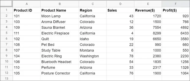
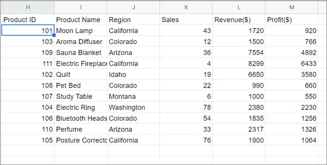
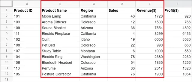
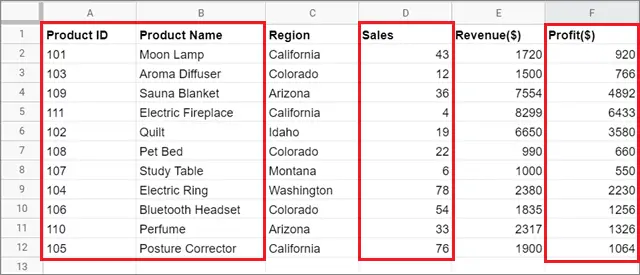
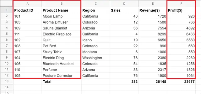
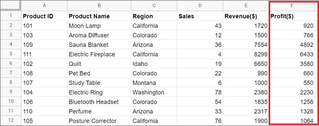
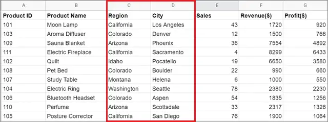
To know about the QUERY function in Google Sheets with a suitable example, we will use this sales figures table of an ecommerce website given below.

Before we begin with the execution of the function, it’s essential to add a simple name to your data for better referencing.

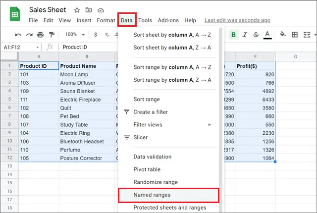
Select the entire data table in the sheet as shown in the figure given below. Then, click on the Data tab in the menu bar and select Named ranges from the drop-down menu.

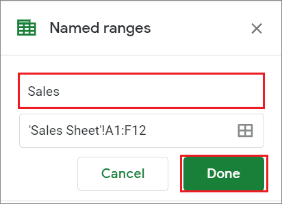
Then, enter a simple name for easy reference. Here, we have named the range as ‘Sales’ in the first blank field. The ‘Sales Sheet’ in the second field is the name of the spreadsheet which we are using for this purpose.

Click on OK once you have entered the necessary information.

Now, the simple syntax for using the query formula in any cell will be as follows:

=QUERY(Sales,“Enter your SQL query in these quotes”,1)=QUERY(Sales,“Enter your SQL query in these quotes”,1)

Instead of Sales, you can also enter the original range, i.e., A1:F12. However, we can use the name of the data range for better referencing.

Also, after you specify the range, make sure to add your query in double quotation marks. Now, let’s look at how to execute different types of commands using the QUERY function.

QUERY Function With The SELECT Clause

If you want to retrieve the entire table in a different set of cells, you can use the SELECT clause for this simple operation. Let’s see how this works.

1. Select The Cell And Enter The QUERY Function

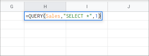
To begin with, select the cell and enter the QUERY function in Google Sheets to retrieve the entire table. We have selected cell H1 in our case.

Here, ‘SELECT *’ tells Google Sheets to select and retrieve the entire table.

2. View The Results

Press the Enter key to view the retrieved table. You can see the entire table has been retrieved starting from column H.

Similarly, you can also retrieve a specific column by replacing the ‘*’ with the column header in the QUERY function. This is how it would look like.

=QUERY(Sales,“SELECT C”,1)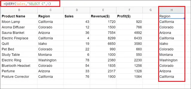

Here, we have retrieved column C in column H using the SELECT clause. You can embolden the column header manually using the Ctrl + B keyboard shortcut to make it look more distinct.

QUERY Function Using WHERE Clause

If you want to retrieve data based on specific conditions, you need to use the WHERE clause in the QUERY function in Google Sheets.

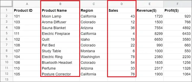
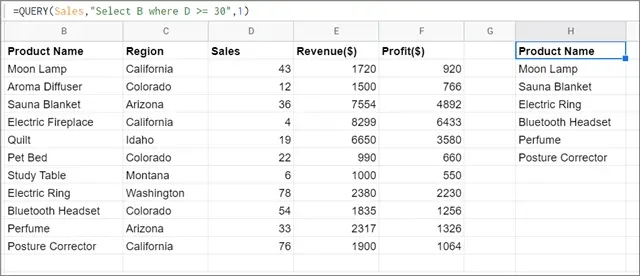
In the sample sales sheet, let’s suppose you have to retrieve the products that have made more than or equal to 30 sales. Here, we will be working with values in columns B and D respectively.

1. Select The Column And Enter The Function

We will retrieve the said result in column H. So, select cell H1 and enter the QUERY language function as given below.

=QUERY(Sales,“Select B where D >= 30”,1)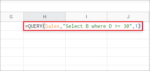

2. View The Result

Press the Enter key to view the result. You can see that the function retrieves data based on the given condition in column H.

QUERY Function Using Multiple Columns And A Single Condition

Let’s say you want to retrieve data from multiple columns based on a single condition in the given sales sheet.

For example, we will retrieve all products that have amassed revenue of more than $5000. We will also retrieve their regions and number of sales respectively. So here, we have to work with columns B, C, D, and E.

1. Enter The Formula

To begin with, select the cell and enter the QUERY function in Google Sheets using the appropriate condition. Here, we have selected cell H1.

The formula will be as given below.

=QUERY(Sales,“Select B, B, D where E>5000",1)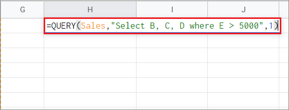

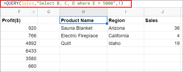
2. View The Result

Press the Enter key to obtain the result in the selected cell. The QUERY function in Google Sheets has successfully returned the cell values based on the given condition.

QUERY Function Using Multiple Columns And Multiple Conditions

In the previous example, there was only one condition for retrieving data. Now, let’s see how we can use multiple conditions with multiple columns for obtaining data.

In this example, we will single out products that have amassed profits of more than $2000  and have made more than 20 sales. We will also retrieve their product IDs. So, in this case, we will be working with columns A, B, D, and F.

1. Enter The Function

We will retrieve the data in column H, so select cell H1 and enter the QUERY function in Google Sheets.

The formula for this condition is given below.

=QUERY(Sales,”Select A, B, where D > 20 and F > 2000”,1)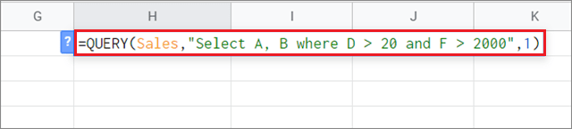

2. View the result

Press the Enter key to obtain the results. You can see the QUERY function retrieves accurate values based on multiple conditions from multiple columns of the data.

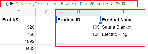
Users can add more than one condition in the function by placing an ‘and’ after the preceding condition.

QUERY Function In Google Sheets Using ORDER BY Clause

The ORDER BY clause is used to sort data into ascending or descending order according to the users’ requirements. This function is always mentioned after the SELECT and WHERE clauses in a QUERY function.

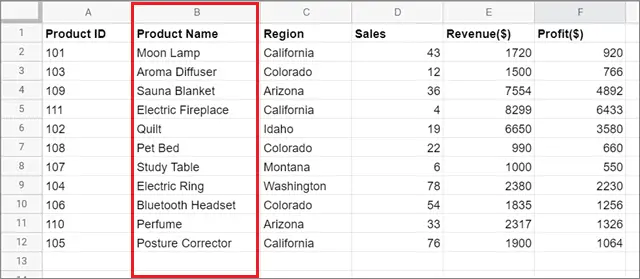
In the given sample sheet, we will arrange the products and their respective details in ascending order. So, here we have to sort the data in column B in ascending order.

1. Enter The ORDER BY Clause

To start with, enter the QUERY function using the ORDER BY clause. In our case, the formula will be as given below.

=QUERY(Sales,“Select A, B, C, D, E, F Order By B ASC”,1)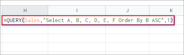

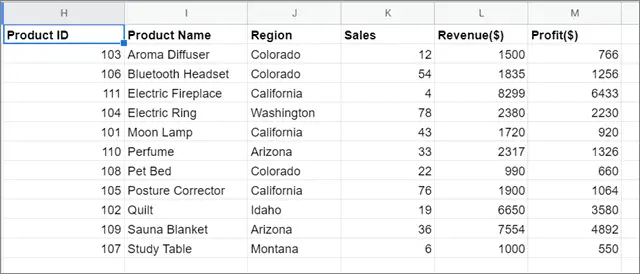
2. View The Result

Now, press the Enter key to obtain the results. You can see the products arranged in ascending order and all other columns sorted according to the order of products.

To arrange the columns in descending order, you can use ‘DESC’ instead of ‘ASC’ in the formula.

By selecting appropriate columns, users can also avoid having a mismatch between them after using the ORDER BY clause.

QUERY Function Using LIMIT Clause

The LIMIT clause is useful when you want to limit the number of results that a function will return. This clause is used after the Select, Where, and Order By clauses in the Google Sheets QUERY function.

We will refer to the result in the previous example. Here, we have eleven products, so let’s limit them to five using the LIMIT clause.

1. Enter The Clause In The Formula

Since we are considering the previous example, we need to add the same formula and add the LIMIT clause in it. This is how the function will look like.

=QUERY(Sales,”Select A, B, C, D, E, F Order By B ASC Limit 5”,1)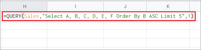

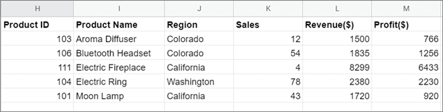
2. View The Result

Press the Enter key to obtain the results. You can see only five results have been returned by the function as specified by the LIMIT clause.

QUERY Function Using Arithmetic Functions

The QUERY function in Google Sheets also allows users to calculate values using the table data. In the sample sheet given below, let’s calculate the percentage of profit owned by each product in the total profit.

We will also display the Product ID and Name in the result along with the percentage profit. So, here we have to work with columns A, B, and F.

1. Enter The Function

This is how the QUERY function in Google Sheets will look like when you enter it in the selected cell.

=QUERY(Sales,”Select A, B, (F/23677) * 100”,1)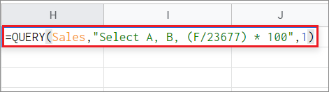

2. View The Result

This is how the result will look when you press the Enter key.

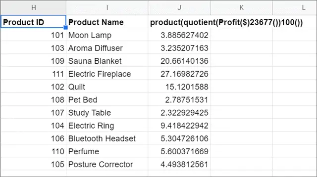
You can use the Format menu in the menu bar to change how the numbers look. However, to rename the header of the percentage column, you will need to use the LABEL clause.

QUERY Function Using LABEL Clause

The LABEL clause is used when you want to name a new column that isn’t present in the selected table range.

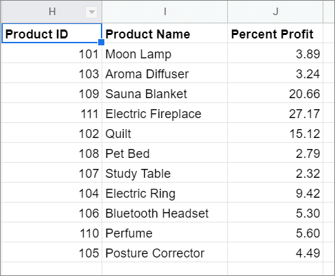
Considering the result in the previous example, we created a separate column for percentage, but we didn’t have a proper column ID for it. Let’s see how we can insert a column identifier for this column.

1. Enter The Function

In this case, the formula will be similar to the one we used in the previous example. The only addition will be the LABEL clause.

=QUERY(Sales,“Select A, B, (F/23677) * 100 LABEL (F/23677) * 100 ‘Percent Profit’ ”,1)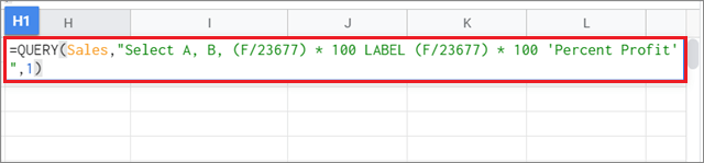

2. View The Result

Press the Enter key to view the results. The column header for the percentage column has appeared as defined by the LABEL clause.

QUERY Function Using Aggregation Functions

The QUERY function in Google Sheets also allows users to know the highest, lowest, and average figures in a dataset.

Let’s consider the sample sales sheet for this purpose. We will calculate the products with maximum profit, minimum profit, and the average profit gained in every sale.

So, here we will work on column F.

1. Enter The Formula

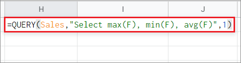
First and foremost, select the cell and enter the formula. This is how the Google Sheets formula will look like.

=QUERY(Sales,”Select max(F), min(F), avg(F)”,1)

Here, max(F) will return the product with maximum profit and min(F) will return the product with minimum profit. The avg(F) function will return the average profit made in every sale.

2. View The Result

You can see the result after pressing the Enter key. Once the figures are displayed, you can identify the corresponding products manually.

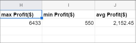
From the result, it is clearly evident that Electric Fireplace is the most profitable product while Study Table has the minimum profit contribution.  

QUERY Function Using GROUP BY Clause

The QUERY Function in Google Sheets using the GROUP BY clause is by far the toughest to understand. However, if you have used the pivot clause in Google Sheets or an Excel workbook, you can grasp it easily.

The GROUP BY clause uses aggregate functions to summarize data which is similar to what a pivot table does in datasets.

Let’s consider the sample sales sheet as an example. Here, we will count the number of cities and group them according to their states. So, we will work with columns C and D in this example.

1. Enter The Formula

The formula, in this case, will be as given below.

=QUERY(Sales,”Select C, count (D) Group By C”,1)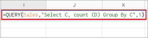

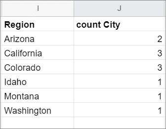
2. View The Result

Press Enter key to view the result.

In this manner, you can use the QUERY string as a substitute for SQL code for editing and summarizing datasets in multiple sheets. You can also use the QUERY function in Google app for Sheets, but we recommend using it on a PC for better convenience.

Along with the QUERY function, the VLOOKUP formula is another important function users need to know for better data analysis.

Conclusion

There are many functions in Google Sheets that help users in performing good data analysis on spreadsheets. However, when it comes to the most important ones, it’s nigh impossible to exclude the QUERY function in Google Sheets from this list. This function allows users to perform database searches like SQL in a Google spreadsheet.

The Google Sheets QUERY might be easy to understand, but you will need to practice it daily to gain a better understanding and a strong command of it. This function is mandatory for all users who are working in the field of data science and analysis.