Google Sheets is the most popular alternative to Microsoft Excel, used for storing statistical and numerical data. If you spend hours working on spreadsheets, it’s essential to know how to use an array formula in Google Sheets to ease data calculation for multiple criteria. A standard procedure gives you a single value, but when it comes to calculating chunks of values, look no further than the Google Sheets or Excel array formula.
For example, let’s consider you have to do calculations for hundred rows in a sheet. To begin with, you will enter the formula in a blank cell and get the result. Then, you will drag the cell down until the last row to get results for all the rows. This is where the array formula comes into play; it cancels out the drag function and calculates multiple values for thousands of rows in the blink of an eye.
How To Use Array Formula In Google Sheets For Faster Calculations
Sometimes, users may also want to link statistical data from one sheet to another in the same Google spreadsheet. If you wish to do the same, check out how to link multiple cells in Google Sheets for better cross-sheet referencing. Let’s take a look at how you can use the array formula to get over a massive number of calculations within seconds.
Note: You can also use the array formula on the Google Sheets app. The process is similar to Google sheets on the PC.
How To Use Array Formula
It’s better to know how to use the multi-cell array formula in Google Sheets with the help of an example. This spreadsheet formula can be used to expand the range of non-array functions in a sheet.
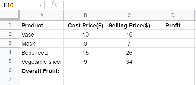
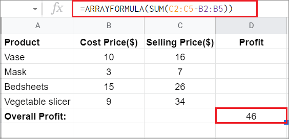
Here, we have a product worksheet where we need to calculate the profit earned from selling each product and the overall profit. Column B contains the cost price, and column C includes the selling price.
Now, let’s get on with the steps.
1. Select The Cell And Enter The Google Sheets Array Formula
To find the profit for all the products, select the first cell in the Profit column. Now, let’s see the syntax for the array formula.
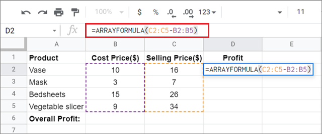
ARRAYFORMULA(array_formula)Here, array_formula is the single formula that we have to use to get the value. In our case, we have to use a subtraction function to get the array result.
Also, make sure you select the entire data range and not just a single cell while using the function.
In our case, the array formula will look like this.
ARRAYFORMULA(C2:C5 - B2:B5)Here, the range of cells C2:C5 considers the selling price of all products, and B2:B5 is the cost price of all products.
Now, enter the array formula in Google sheets involving column B and column C in the sheet, as shown below.
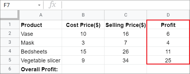
Press the Enter key to obtain the array result. You can see the profits for all products appear in the cells.
2. Use The Array Formula For Calculations Containing Multiple Functions
Now, it’s easy to calculate the overall profit once you have the earnings for each product. But, let’s suppose you have to calculate the overall profit directly.
In this case, you need to use the sum function and the subtraction function in an array formula.
So, according to the given condition, our formula for this case will be as shown below:
ARRAYFORMULA(SUM(C2:C5-B2:B5)Now, enter this formula in the selected cell.
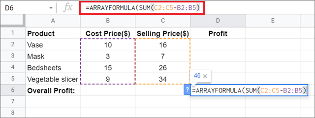
Press the Enter key to obtain the overall result.
An Alternative Way To Use Array Formula Function In Google Sheets
If you don’t like entering the full syntax of the array formula in Google Sheets, you can use a helpful hack to overcome it.
Once you select the cell in which you want the result, just type the functions you want to use and press the Ctrl+Shift+Enter keyboard shortcut. Doing so will automatically add the array formula wrapper to your operation.
If you are a Mac user, you need to press the Cmd+Shift+Enter key combination to avail of this feature.
Then, you can press the Enter key to obtain the required results.
Use the Array Formula with IF Function In Google Sheets
Sometimes, we often across certain datasheets where we need to single out terms and values based on specific criteria. The IF function in Google Sheets allows users to sort their data quickly.
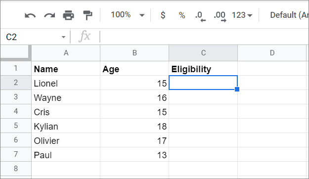
For example, let’s take the datasheet above. Here, you have to sort out boys according to their ages for a tournament. Boys of age 17 and above are eligible to play the game. Let’s see how the IF function in Google Sheets helps us in this case.
1. Select The Cell And Enter The Array Formula Function
First, select the cell and then enter the equation according to the given criteria using the IF function.
In our case, the equation will be as given below.
=ARRAYFORMULA(IF(B2:B7>=16, “Yes”, “No”))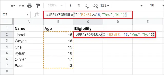
Here, B2:B7 is the range of ages of the boys; Yes and No are the answers you wish to generate in the column next to the range of ages.
2. Obtain The Results
Once you press the Enter key after entering the array formula in Google sheets, you will see the results appear in the Eligibility in the column.
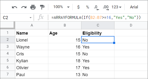
To enhance the look and enable users to point out cells quickly, you can do conditional formatting to turn a particular data point into a different color so that they are quickly visible.
How To Use Array Formula With Text Function In Google Sheets
Now that we know how to use the Google Sheets array formula with statistical data, let’s check how to use the text function in Google Sheets with array formula.
When it comes to text, we usually use the array formula function to combine data from two or multiple columns into a single column.
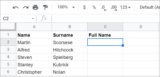
In the above datasheet, we have to combine names and surnames from columns A and B in column C.
1. Create And Enter The Formula
To begin with, create the formula for amalgamating the terms from columns A and B. In our case, this is how the formula looks.
=ARRAYFORMULA(A2:A6&" "&B2:B6)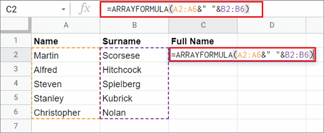
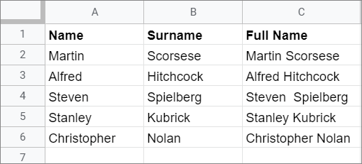
2. See The Results
After you have entered the formula, press Enter key to see the results.
If you wish to separate the terms back again, you can check out how to split the text into columns in Google Sheets.
How To Use Horizontal Arrays
Until now, we have seen how to apply the Google Sheets array formula for vertical arrays. Let’s check out how to do the same for horizontal data.
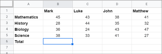
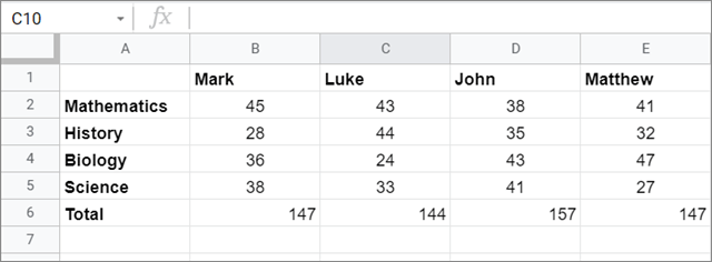
Here, we have a list of students and the marks they have obtained in particular subjects; the main idea is to calculate the total marks of each student by using a horizontal array formula in Google sheets involving multiple rows.
1. Enter The Formula In Column
To start with, select the cell and enter the formula as follows.
=ARRAYFORMULA(B2:2+B3:3+B4:4+B5:5)
Now, notice the difference in the selection of cell range. The range B2:2means we have commanded Google Sheets to consider the entire blank row of B2 instead of entering B2:B5and selecting individual cells in the entire column.
2. Press Enter Key And View The Display Of Values
Once you form the equations for each row number and add them in the formula, press the Enter key to see the results. You will see that the total of all four students appears in the Total row.
How To Use Array Formula In Multidimensional Arrays
In this section, we will see how the Array Formula in Google Sheets can be used in cases where you need to calculate values in tables. Make sure you leave cell A1 blank if you are creating a table of such kind.
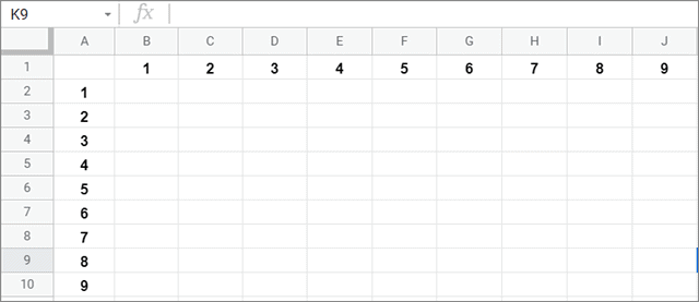
1. Enter The Formula
A table uses both vertical and horizontal orientations, so you need to create a formula accordingly. In the given table, we have to obtain the multiplied results of the values in the horizontal and vertical cells.
The formula will be as follows.
=ARRAYFORMULA(A2:A10*B1*J1)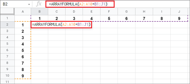
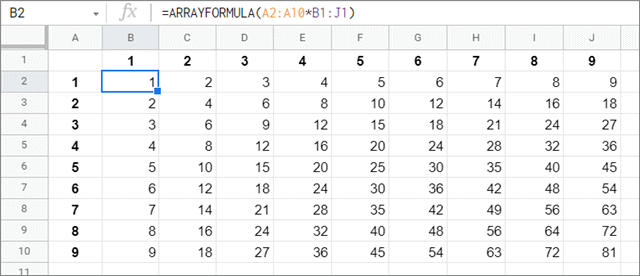
2. Press The Enter Key To See The Results
Now, press the Enter key to view the results of the formula applied to the data range. You will see the entire table gets filled with accurate values in the blink of an eye.
You can also use the array formula with the VLOOKUP function in Google Sheets for data analysis. If you don’t have a PC to work on, you can use the array formula in Google Sheets app; the process of using the procedure is similar to how we use it on the PC.
Conclusion
Google Sheets offers a wide variety of formulas for the ease of doing calculations. If you are working with multiple sheets and huge chunks of data and need to do scores of calculations, you can go for the array formula in Google Sheets. Using this custom function, users can save valuable time that would otherwise be required to calculate data manually.
Apart from being a time savior, the Google Sheets array formula function is also pinpoint accurate with the results it provides, thereby improving the efficiency of data in the spreadsheet. Also, the array formula function is available in both Google Sheets and a Microsoft Excel spreadsheet.


