Working on a large Google spreadsheet or Microsoft Excel can be knotty at times. To add to your misery, what if the datasheet is disorganized! Such conditions are never a good omen if you are having a race against time and want to complete your work quickly. Pivot table in Google Sheets can help you in such circumstances.
When your spreadsheet keeps getting larger each day, a Google Sheets or Excel pivot table can help you manage and summarize data swiftly and deliver the results you need. In a nutshell, a pivot table helps you gather values from random cells in a spreadsheet and summarize them in an instant. If you have duplicate values in your spreadsheet, you can know how to remove duplicates from Google Sheets.
How To Create, Edit And Use Pivot Table In Google Sheets
Suppose you are working on a complex datasheet. In that case, a Google Sheets pivot table can help you single out smaller pieces of information and derive meaningful insights and conclusions by performing various actions on them. Let’s take a look at the process of creating a pivot table in Google sheets.
4 Steps To Create Pivot Table In Google Sheets
1. Select the range of cells in Google sheets.
2. Click on the Data tab and select the Pivot table option.
3. Set the preferences and click on Create.
4. View the pivot table.
We can create a pivot table using the four steps mentioned above. Now. let’s take a look at these steps in detail with images.
How To Create A Pivot Table In Google Sheets
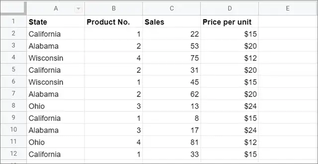
Let’s understand the pivot table in Google sheet report using a sales table sample listed below. The table consists of four columns that denote State, Product Number, Sales, and Price per unit.
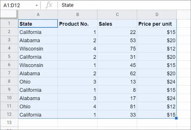
1. Select the cells
To begin with, select the data range in the datasheet. However, make sure that the selected cells in the pivot group have associated column headings for creating a pivot table. Also, if you wish to select the entire dataset, you can click on the box in the top left corner of the existing sheet.
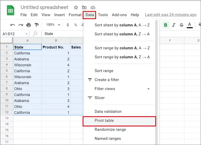
2. Create the Pivot table
Click on the Data tab in the Menu bar and select the Pivot table option from the drop-down menu.
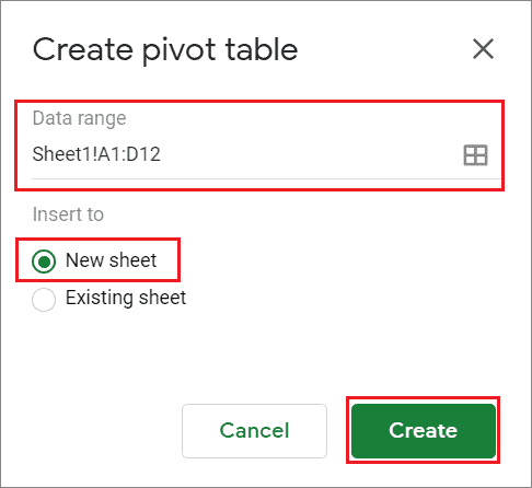
3. Set the preferences and click on Create
Next, you will see a dialog box that will ask you to confirm your cell range selection. You can also select whether you want the pivot table on the original datasheet or a new sheet.
Click on Create once you set the preferences.
4. View the pivot table data
The pivot table in Google Sheets will open automatically. If it doesn’t, you can click on the Pivot Table sheet in the tab bar at the bottom.
How To Edit A Pivot Table
Once you open the Pivot table in Google Sheets, you can see the pivot table editor window in the right sidebar. Let’s get to know what the sidebar consists of.
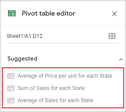
The Suggestions section at the top of the sidebar offers suggestions based on the information you have chosen in the sheet. You can click Add button in that section to create the pivot table as per the parameters set by Google Sheets.
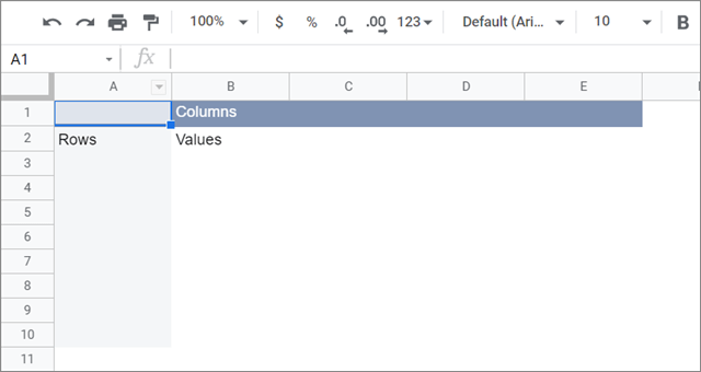
Next to the suggestions, you can add four fields using the pivot table editor: Rows, Columns, Values, Filters.
Rows: Adds all unique items of a specific column from your data set to your pivot table as row headings. They are always the first data points you see in your pivot table in light grey on the left.
Columns: Adds selected data points (headers) in aggregated form for each column in your table, indicated in the dark grey along the top of your table.
Values: Adds the actual values of each heading from your dataset to sort on your pivot table.
Filter: Adds a filter to your table to show only data points meeting specific criteria.
1. How to Select Rows and Columns to create a pivot table format
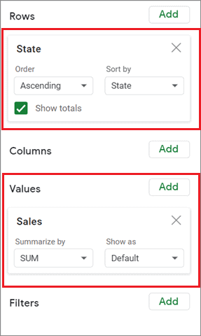
Considering the above example, let’s assume that you have to calculate the total number of sales made by each state. Click on the Add button in front of the Rows section. You will see the parameters we have used in the table.
First, select the State column in the Rows section.
Then, since we need to find out the number of cells, select the Sales column in the pivot table Values section. In that tab, select SUM in the ‘Summarize by’ section.
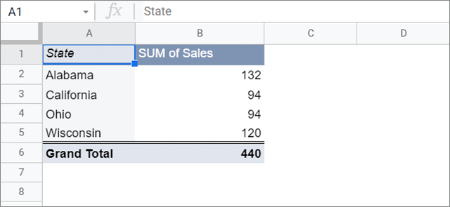
This is how the result would look like when you complete the operation.
2. How to work with multiple values
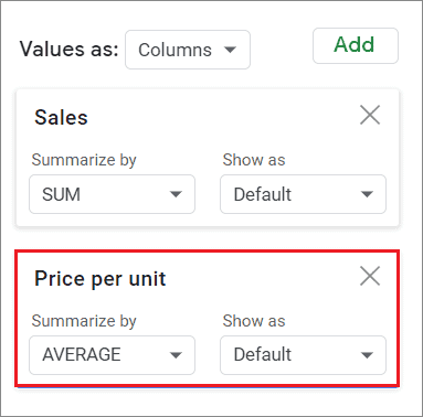
You can work with multiple values in the same pivot table in Google sheets. For example, let’s calculate the average revenue made by each state.
Click on the Add button in the Values section and select the Price per unit column. Then, select the AVERAGE function in the ‘Summarize by’ section.
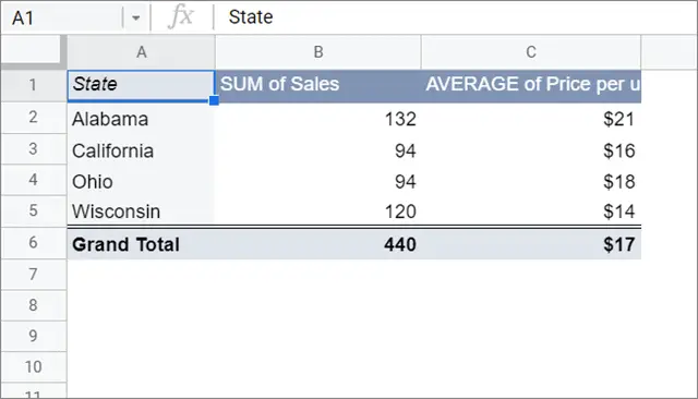
Check how the table looks like once you add the preferences.
3. How to work with multiple categories
Pivot table in Google Sheets also allows users to obtain data insights for multiple categories in a dataset consisting of thousands of rows. Let’s assume that you are asked to get the total number of sales and the average revenue of product category number 1 made by the state of California.
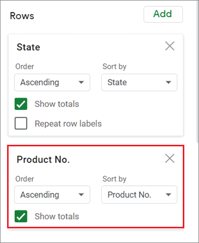
To proceed further, add the Product number tab in the Rows section.
You can see the number of products and their sales and revenue figures in the table given below.
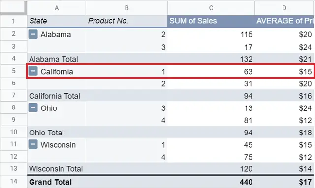
Here, we can quickly figure out that California has made 63 sales of product 1 with average revenue of $15 per unit.
4. How to filter data in Pivot tables
Now, what if you want to make the data look more precise? For example, let’s assume that you have to display the figures only for product 3 in all the states.
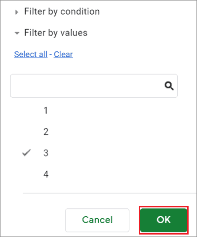
To do that, go to the pivot table Filters tab and Product No. as the parameter. Then, unselect all the other product numbers as shown in the figure given below.
Now, view the results.
You can also filter data based on specific values or conditions. For example, let’s assume you have to display the number of products that have made 50 or more sales.
To begin with, first select the Sales column in the Filters menu.
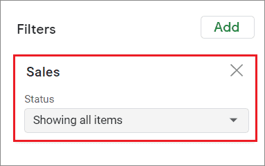
Now, click on the Status section and choose the Filter by condition option. Then, select the Greater than or equal to option from the drop-down menu.

Now, enter the value of the condition. Here, we will enter ‘50’ as per the conditions assumed above.
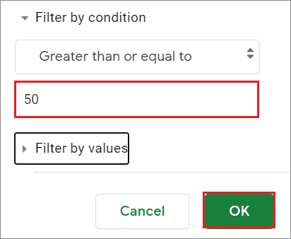
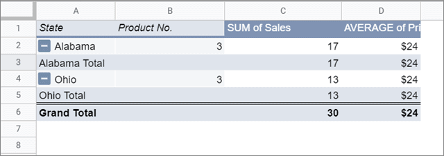
You can view the results as shown in the image given below.
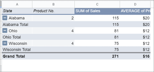
While reading the insights, make sure you don’t get confused with the Total figures of each state; these figures aren’t considered while filtering data.
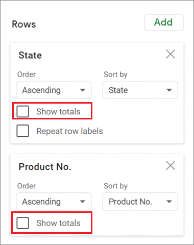
If it’s confusing, you can switch off the Show total option from the Rows section.
5. How to make your formula
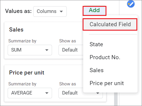
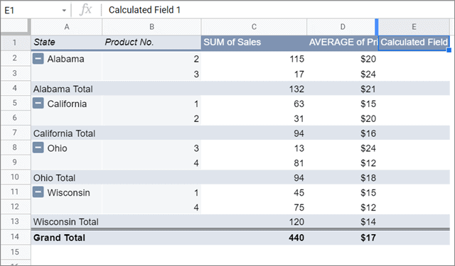
Suppose you are not satisfied with the operational functions or use a formula that isn’t available in the given function. In that case, you can create one using the Calculated Field option.
In the Values section, click on the Add section and select Calculated Field.
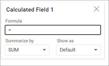
Now, enter the custom formula in the data field.
You can see that the Calculated Field is displayed in a separate column in the table. Likewise, you can add multiple pivot table columns of Calculated Fields as per your requirements.
To use the pivot table in Google Sheets for data analysis, it’s essential to know how to perform different types of calculations on the given data. Conditional formatting in Google Sheets also helps users arrange pivot tables and displays only the pivot table values required.
How To Copy And Paste Pivot Tables In Google Sheets
Once you have created a pivot table with all the required formats containing all the necessary values, you can save it separately using the copy-paste function.
1. Select the cells
You can either select the cells used in the pivot table or the entire Google Sheets spreadsheet by clicking on the box in the top left corner.
2. Use the keyboard shortcut for copy-paste function
If you are a Windows user, press the Ctrl + C shortcut key and paste the pivot table in another sheet by pressing the Ctrl + V shortcut. Make sure you have enough cells to fit the data in the spreadsheet.
If you are a Mac user, use Cmd + C to copy the pivot items in the clipboard and Cmd + V to paste values in a different sheet. Also, you need to remember that pivot tables cannot be created on the Google app for Sheets; you need to work on the desktop versions for this purpose.
Conclusion
Working with complex datasheets can be a real problem if you are unaware of the necessary features that can help you reduce your workload. A pivot table in Google Sheets is one such facility that eases the burden of summarizing data that you have entered randomly in a spreadsheet.
Pivot tables offer many advantages, but only those that are related to summarizing data. There aren’t too many options for carrying out complex calculations, which may compel you to perform this manually. Also, creating this task isn’t necessarily a child’s play for every user; you need to practice using pivot tables daily to get a proper hang of how to use it in different scenarios.


