How To Use Concatenate in Google Sheets To Link Cells

Google Sheets is the go-to spreadsheet program for number-crunching for many users. The internet alternative of Microsoft Excel offers various functions, much like its competitor, to make data calculations as easy as falling off a log. One such feature is about getting to know how to use the CONCATENATE in Google Sheets.

The CONCATENATE function links data from multiple cells together and stores it in a single cell. Apart from the concatenation formula, you can also use the CONCAT and JOIN functions to combine cells in Google Sheets. These functions vary on the scale of difficulty but exist to provide the same facility; they help in merging data so that large data sets become easily manageable. You also need to link cells in Google Sheets while using the CONCATENATE function.

How To Use CONCATENATE Google Sheets Function

To better comprehend, we will first start with the CONCATENATE function, followed by the CONCAT and JOIN functions, respectively. Let’s get to know how to use these features to combine data and link individual cells in Google Sheets.

Details for CONCATENATE in Google Sheets

Now that you have understood the basics of using the CONCATENATE in Google sheets; let’s check out the process in detail with images for better comprehension.

1. How To Use The Basic CONCATENATE Function In Google Sheets

CONCATENATE in Google Sheets offers more flexibility than what we saw with the previous function. You don’t need to add any extra or additional spaces to show separation in the linked data, as you can use the operators for that purpose.

Step 1. Enter the CONCATENATE formula

The Google spreadsheet given below consists of parts of a pace name scattered across multiple columns. We will use the CONCATENATE in Google Sheets to combine the cell contents.

The basic syntax for this formula is given below.

=CONCATENATE(string 1, string 2,...)

To begin with, enter the function as shown in the image below.

=CONCATENATE(A2,B2,C2)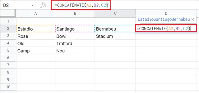

You can also use the ampersand symbol(&) instead of the comma(,) to combine data from separate cells.

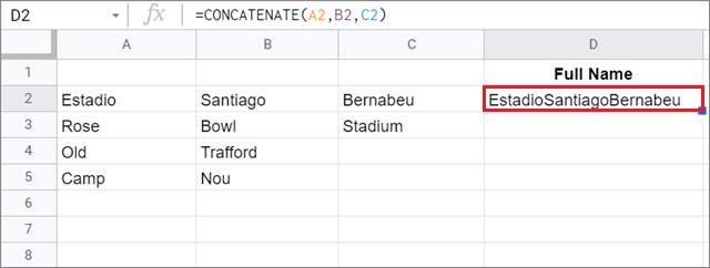
Step 2. Press the Enter key to obtain the results

Now, press the Enter key to calculate the results. This is how the value in D2 should look like.

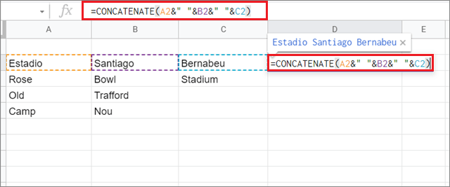
Insert space character in the CONCATENATE function

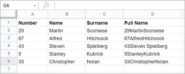
The results above aren’t perfect because you need to insert spaces between terms from different columns so that the name is distinguishable and easy to read.

To insert space, use the following formula.

=CONCATENATE(A2&” “&B2&” “&C2)

The ampersand(&) acts as the connector, and the space character (“ “) indicates the space that needs to be left out after a particular term.

Now, press the Enter key to get the results in a different cell.

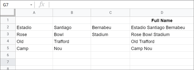
Once you get the result in the first cell, use the drag function to apply the formula to the remaining cells and obtain results for the same.

2. How To use the CONCATENATE Function With Line Break

A line break allows the combined cells in Google Sheets to be aligned one below the other. Here is the specific function for inserting a line break.

=CHAR(10)

In the Google sheet image given below, we have to compile an address by combining the data from multiple cells using the line break function.

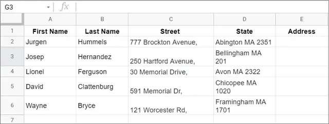
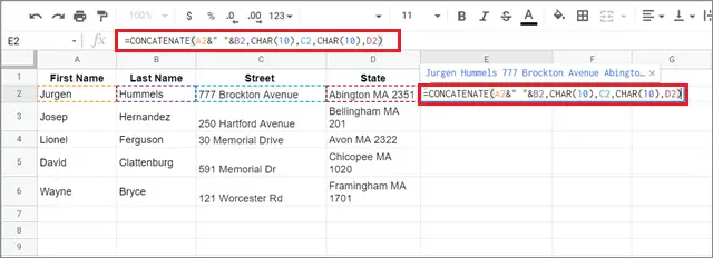
Step 1. Enter the CONCATENATE formula with a line break

To begin with, open the spreadsheet and enter the formula for CONCATENATE in Google Sheets as given below.

=CONCATENATE(A2&” “&B2,CHAR(10),C2,CHAR(10),D2)

The A2&” “&B2 term is used to keep the names together in the same line. The line break function after B2 will place the content in cell C2 under the name.

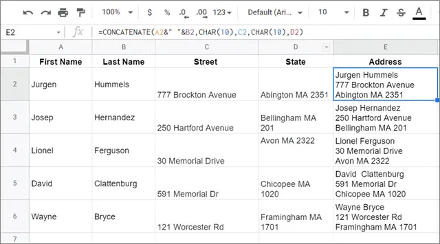
Step 2. Obtain the results

Press the Enter key to get the results of the function. You can use the drag function to obtain results for all cells once you get the result in the first cell.

3. How To Use The CONCATENATE Function With Running Numbers

Running numbers means assigning the number format in ascending order to successive cells. You can do this by using the CONCATENATE in Google sheets.

In the datasheet given below, we have to combine cells of the first and last names and display the multiple values in cells of column C. Along with that, we also have to assign numbers from 1 to all the names.

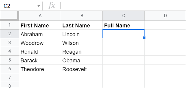
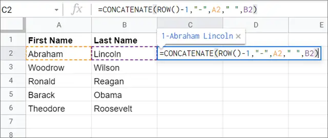
Step 1. Enter the formula for running numbers

The formula for running numbers is given below.

=CONCATENATE(ROW()-1,”-”,A2,” “,B2)

Here, the term ROW()-1 indicates the running numbers that will be assigned to the terms.

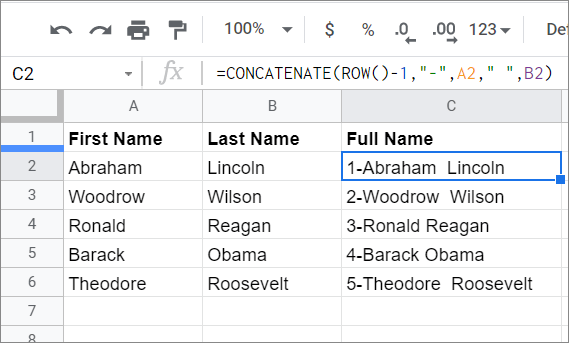
Step 2. Press the Enter key to get results

Now, hit the Enter key to calculate the results. Once you get the result in the first cell, you can either use the drag function to apply the formula to all the subsequent cells or choose the Suggested Autofill option that appears after you press the Enter key.

4. How To Use the CONCAT Google Sheets Function

The CONCAT function is the easiest way to combine data from two cells, but it has two shortcomings. First, it can combine data from only two cells, and secondly, it doesn’t allow the use of operators to decide how the linked data should be displayed.

The basic syntax for the CONCAT formula is given below.

=CONCAT(string 1, string 2)

Step 1. Select the cell and enter the formula

To begin with, open your data spreadsheet and select a blank cell in which you want to display the linked data. Here, we will combine names and surnames from two cells into separate cells using CONCATENATE in Google Sheets.

Enter the formula given below in the blank cell.

=CONCAT(A2,B2)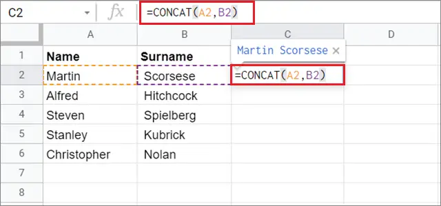 

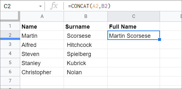
Now, make sure you notice that all the values from cells of column B start with a blank space. This is an adjustment you have to make as the CONCAT formula in Google Sheets doesn’t allow the use of operators to insert spaces between cell data.

Step 2. View the results

Now, once you press the Enter key, the compiled data will appear in column C.

5. How To Use The JOIN Function

The JOIN function in Google Sheets is also one of the best features to use if you’re working on large datasheets. The standout feature of this function is that it allows users to specify the common operator, also known as a delimiter, that needs to be applied after each term present in the formula.

Let’s understand it using an example. Here is an example of CONCATENATE in Google Sheets. Notice how we need to use the comma (,) after each term to connect them.

=CONCATENATE(A2,B2,C2)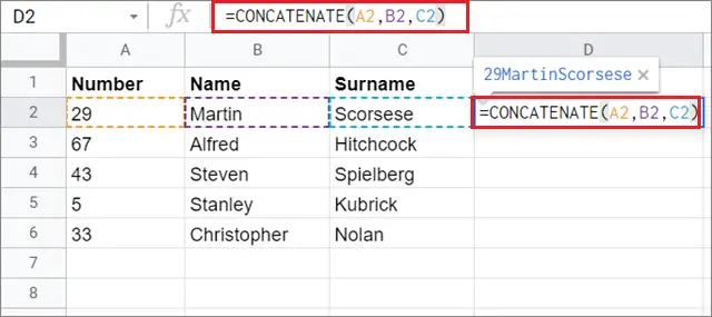

Check the results of the CONCATENATE function in Google Sheets. The contents of cell A2, cell B2, and cell C2 will appear in D2.

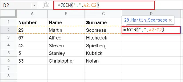
Now, here’s how the same formula can be written using the JOIN function. The common syntax for this function is JOIN(“delimiter”,range).

The JOIN function formula for the above equation will be as given below.

=JOIN(“,”,A2:D2)

Here, the comma(,) string in double-quotes is the delimiter – the operator that needs to be applied after every term in the range of values. The A2:D2 text string is the range of cells to which the function in Google Sheets is to be applied.

Press the Enter key to apply the results. You can use the array formula along with the CONCATENATE function to produce the results for all the cells.

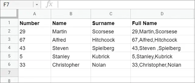
It is crucial to remember that the JOIN function always works with an entire cell range and not single cells, so it is the best function for extensive datasheets. You can also add multiple cell ranges in the same formula if you want to use the same delimiter across those ranges.

6. How To Split Text Cells In Google Sheets

If you have linked all the cells and want to bring them back to their original state, you can use the split function in Google Sheets. You can follow the detailed guide on how to split text to columns in Google Sheets.

Conclusion

Linking cells with data in Google Sheets is a common requirement for many users. Hence, it is necessary to know how to use the CONCATENATE in Google Sheets to manage large data sets better. While there are multiple ways to carry out these tasks, the Concatenation operator is primarily used for this purpose.

You can also link cells in Google Sheets together by using equations that contain the ampersand character(&) as shown above. The CONCAT function is the easiest to use, followed by the CONCATENATE and JOIN functions, respectively. You can also use the QUERY function to combine columns in Google Sheets. However, in the end, the choice of using the formulas rests with the users.