How To Use Conditional Formatting In Google Sheets

Google Sheets is widely used for number-crunching and is an acceptable alternative to Microsoft Excel. Of all the features it offers, none is perhaps as important as those related to conditional formatting. When users know how to use conditional formatting in Google Sheets, they can apply specific formatting to the cells that meet the set criteria.

Conditional formatting entails coloring separate Google Sheets cells for highlighting data that needs to stand out in the chunk. This method is also a good alternative for gaining insights and data validation compared to pivot tables, which are used to summarize extensive datasheets. Highlighting data also makes it easy for users to navigate through a complex datasheet. Before conditional formatting, you can also use the VLOOKUP formula in Google Sheets to complete the data analysis.

Conditional formatting can also be used to highlight duplicates. However, you can know how to remove duplicates in Google Sheets if you don’t want them.

How To Do Conditional Formatting In Google Sheets

Conditional formatting might appear very basic as a beginner. But the more you study how to use it in large datasheets, the more complex it becomes. Let’s look at a few ways to apply conditional formatting in Google sheets.

Now that you are well aware of using the basics of conditional formatting in Google Sheets, let’s check out the process using detailed images.

1. Select A Range

To begin with, the basics, let’s see how we can select a range in Google Sheets using conditional formatting.

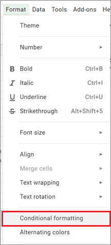
Open conditional formatting from the Format menu

Click on the Format tab in the menu bar and select conditional formatting from the drop-down menu.

Another way to open it is to select the cell range, right-click on it, and choose the Conditional formatting option from the drop-down menu.

Select a data range

Once you open the conditional formatting toolbar on the right side window, enter a range of cells or a single cell in the Apply Range box.

For example, if you want to enter a cell range including all cells from A2 to A11, you can enter it in the format.

A2:A11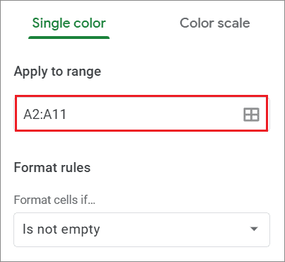

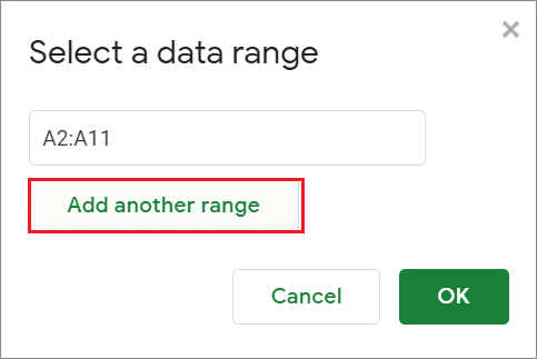
Add multiple cell ranges

You can add multiple ranges by clicking on the table icon situated to the right of the Apply Range box.

Doing so will open a dialog box where you can click the ‘Add another range’ button and enter another range. Click on OK to confirm your selection.

2. Select A Style

Once you have selected a cell range, choose the colors you want to indicate the cells with. You can do this by choosing any color under the Formatting style section.

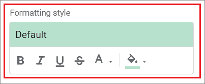
You can also create a custom style by using options like Bold, Italic, Underline, and Strikethrough.

How To Use The Formatting Rules

1. Use The IF Cause

The IF cause is the main feature that allows users to define conditions for conditional formatting in Google Sheets. The first and the primary way to format text using the IF cause is the empty/not empty method.

Select the cells

To begin with, choose a cell or range of cells to format.

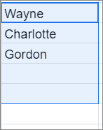
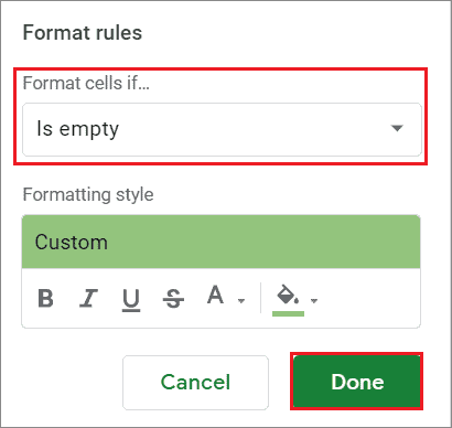
Select empty or not empty option

Once you have selected a range of cells, choose whether you want to format them if they are empty or not. We have decided to format cells and fill them with green color if they are found empty.

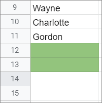
See the result

You can see that the blank cells in the selected range are filled with the chosen cell color.

If you wish to delete the conditional formatting, select that particular cell first. Then, open the formatting toolbar on the right side and click on the Trash icon to delete the formatting settings.

You can also use the Ctrl + keyboard shortcut for Windows PC or Command + for Mac to delete all the formatting applied to a cell in Google Sheets.

2. Conditional Formatting With Text Options

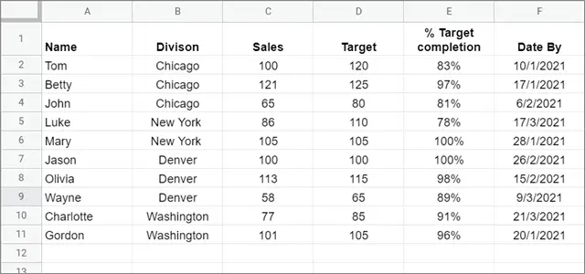
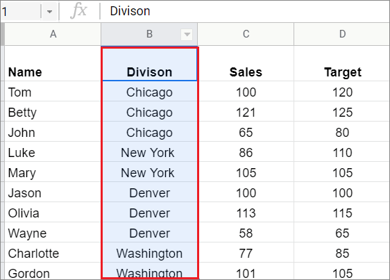
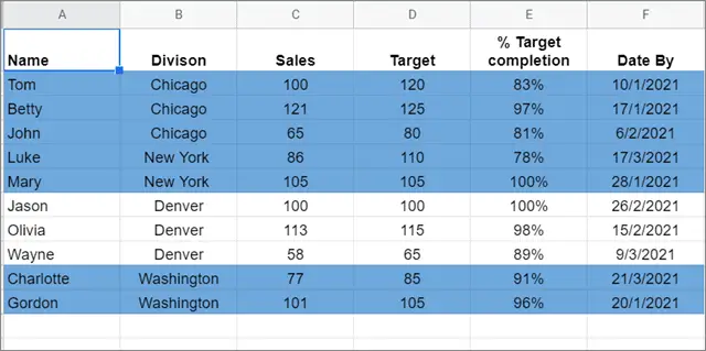
You can also do conditional formatting in Google Sheets based on the text entered in the cells. Let’s check out the simplest way to do it. We will use this sales table below to know how to do conditional formatting in Google Sheets in different ways.

Select the cell range

Once you have opened the conditional formatting sidebar, choose the range of cells you want to work on.

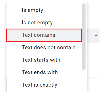
Choose the Text contains option and enter text

There are various ways available for text formatting in Google Sheets. For this example, we have selected the ‘Text contains’ option in the ‘Format cells if’ box. By choosing this option, you can highlight all the cells that contain the text you have specified for formatting.

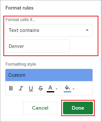
Now, say you want to highlight the sales executives working in a particular division. You can enter the name of the division in the Format cells if box.

In this case, we have chosen to highlight the executives working in the Denver division. Click on Done after you have selected the preferences.

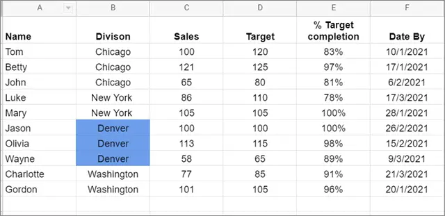
View the results

You can see the cells with the given term are highlighted in the Google Sheets spreadsheet.

Other options for text formatting are Text does not contain, Text starts with, Text ends with, and Text is exactly.

3. Whole Row Formatting

We have seen how to do conditional formatting in Google Sheets based on text. However, the said method highlights only the cells with the selected text.

What if you wanted to highlight the entire corresponding row in which this text appears? This is where you need to use a custom formula to get the required formatting. Let’s work this out on the example given below; the aim is to highlight all the rows that have the word ‘Denver’ in it.

Select the cell range

Once you highlight the main cells with text, click on the Add another rule button in the sidebar.

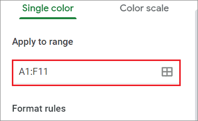
Then, select the entire table by entering the cell references in the ‘Apply to range’ box. Here, the cell references are A1:F11.

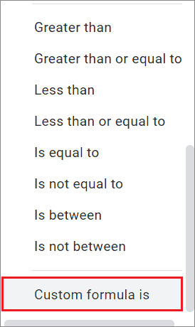
Choose Custom formula option

In the Format cells if section, choose ‘Custom formula is’ from the sidebar.

Enter the formula

Now, enter the formula given below to highlight all the rows containing the text.

=$B1="Denver"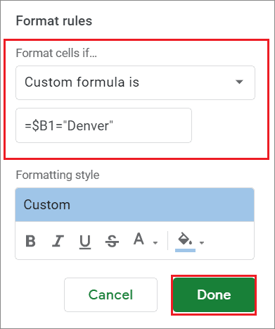

This is how the table should ideally look like once you enter the correct formula.

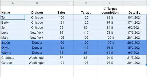
Next, let’s look at how the formula works. The ‘=’ part in the equation that marks the beginning of the formula. B2 is the sample data for the column. The sign ‘$’ before B2 tells Google Sheets to look only at column B. If you put another ‘$’ sign after B2, Google Sheets would only highlight the given term if it appears in a cell in column B and the second row.

However, we only need to lock the entire column B for sample data at the moment, so we don’t need to insert the ‘$’ after B2. Next, you have to insert the term you want to highlight in the double-inverted commas. This tells Sheets the exact text it should look for.

4. Highlight the terms excluding the given text

Suppose you have to highlight text in all rows and columns except those that contain the text ‘Denver’. You need to tweak the formula a bit. To begin with, first, delete the conditional formatting rule that you just applied to the table. Then, add a new rule and enter the given formula.

=$B1<>”Denver”

This is how the result will look like after applying the formula above.

The ‘<>’ symbol is inserted to ask Google Sheets to exclude the text given in the formula from the Conditional format rule.

4. How To Do Conditional Formatting Using Numbers

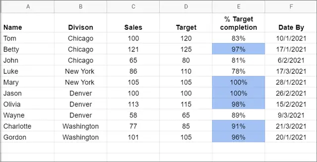
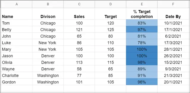
Apart from text, you can also perform conditional formatting in Google Sheets using numbers. In this example, we will aim to highlight all the executives who have completed equal to or more than 90% of their targets.

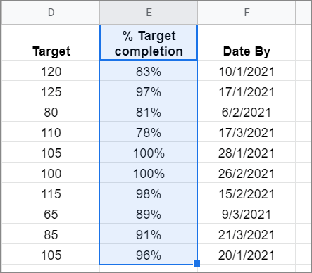
Select the column for conditional formatting in Google Sheets

To begin with, select the range of cells that you wish to work on. Here, we will select column E that contains the percentage of target completion.

Select the formatting options

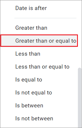
Next, select Greater than or equal to from the drop-down menu in the ‘Format cells if’ dialog box.

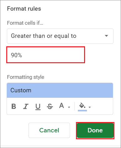
Enter the threshold number

Choose the threshold number, 90% in this case, and click on Done to apply the formatting.

This is how the table should look once you follow all the steps.

Perform conditional formatting on rows

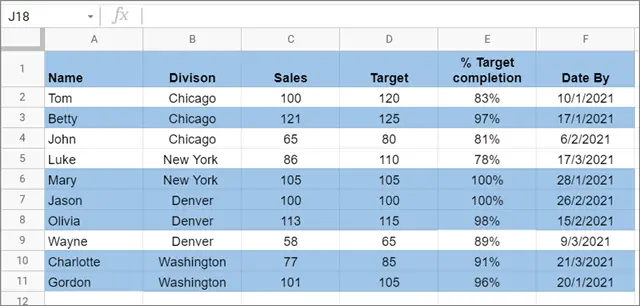
To apply formatting to all the rows that contain a cell value greater than or equal to 90%, you can use the custom formula given below.

The method to apply the custom function is the same as we saw in the previous sections.

=$E1>=90%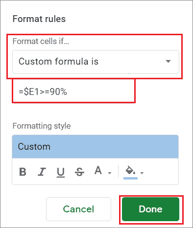

View the result once you have applied the formula.

Do conditional formatting with color scale

Now, if you wish to highlight cell ranges containing numerical values with different colors in a given cell, you can use the background color scale to do it.

Once you have highlighted the first range(here, all the percentages equal to and greater than 90), select the Color scale in the conditional formatting menu.

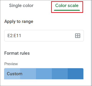
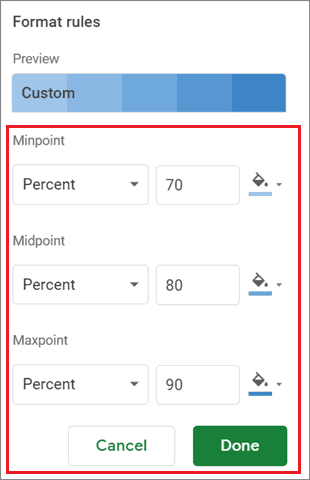
Now, you can choose a Minpoint, Midpoint, and Maxpoint to segregate numbers in a particular numerical range and represent them with different colors.

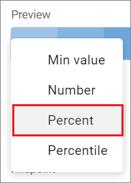
Select the unit for representing the three points; it could be either a minimum value, percentile, number, or percent. Here, we have selected percent.

In the boxes next to the three points, enter the numerical ranges and then choose the color to represent each range.

Click on Done to view the final result.

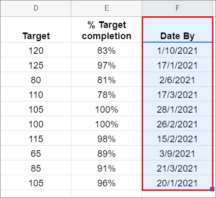
5. How To Do Conditional Formatting With Dates

Sometimes, you might need to do conditional formatting in Google Sheets based on the dates entered in the spreadsheet. Before, you start with this process, defining a particular format for representing dates is necessary.

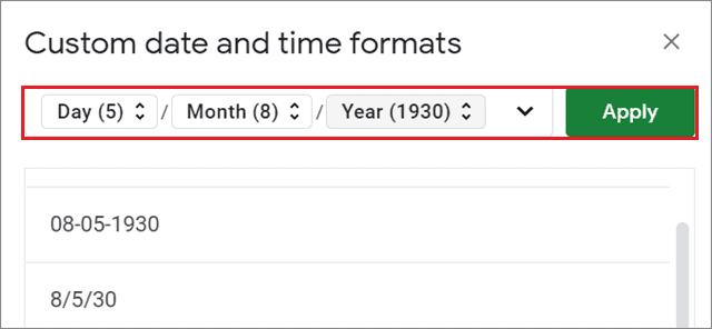
To do so, click on the Format tab, select Number, and choose More date and time formats.

Then, enter the date format that you are comfortable reading with and click on Apply.

Once you have decided the date format, make sure the dates entered in the columns comply with the selected format. Now, let’s move on to the conditional formatting process.

Select the column

To begin with, select the column that contains dates and open the conditional formatting sidebar.

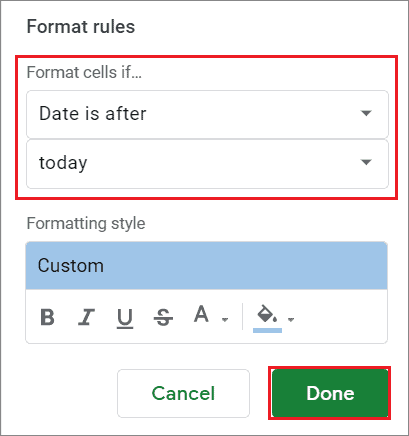
Select the Date option

Now, choose any option related to sorting dates in the ‘Format cells if’ tab. You have three options for formatting sheets based on dates: Date is, Date is before, and Date is after.

Here, we will highlight all the executives who have achieved their respective sales numbers after the current date. The current date is 21 March.

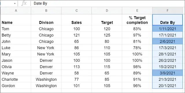
View the results

Once you carry out these steps, you can check the results.

6. How To Do Conditional Formatting Based On Another Cell In Google Sheets

Google Sheets also allows users to format cells based on different cell values. Let’s see how we can do it using the same example above.

The main aim here is to highlight the names of the executives who have more than a hundred sales.

Select the cells

To start with, select the column to work with. Here, we have to highlight the names of executives, so we will select column A.

Select and enter the custom formula

Open the conditional formatting sidebar and select Custom formula from the dropdown list of the ‘Format cells if’ field.

Now, enter the formula given below. Cell C2 represents column C(Sales) in the sheet.

=C2>100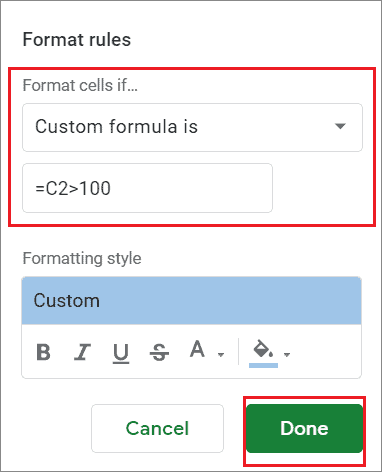

View results

Once you enter the formula, click on Done to obtain the results.

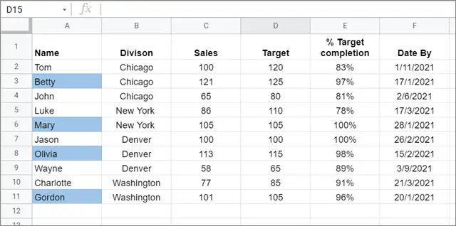
You will see that the selected color has highlighted the names of the executives.

7. Google Sheets Conditional Formatting Based On Values From Other Sheet

Users can also do inter-referencing between multiple sheets in the same file. However, this method contains a complex formula that you need to enter correctly to carry out this process successfully.

Determine the two sheets you wish to work on

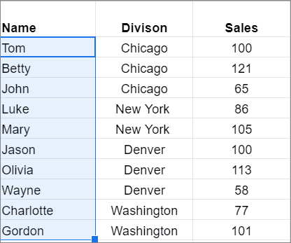
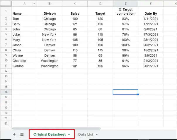
Make sure you have the two Google spreadsheets ready before you begin with this method. Here, we want to highlight the data similar to column B in the Data List spreadsheet into the Original Data spreadsheet.

This is how the Original datasheet looks like:

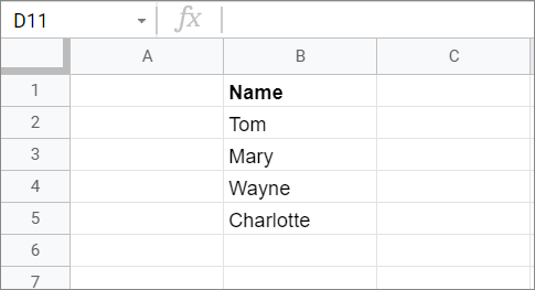
And, this is how the second Google sheet, i.e., the Data List spreadsheet, looks like –

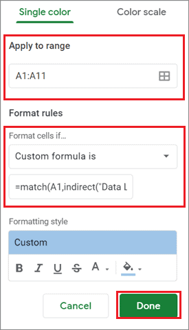
Highlight the cells in the first datasheet and enter the formula

Our job is to highlight the terms in column A of the Original Datasheet that matches with column B in the Data List sheet.

To begin with, open the conditional formatting pane in the Original Datasheet and select the appropriate column to work with. Here, we have selected column A.

Then, choose ‘Custom formula is’ in the conditional format rules field.

Next, enter the given formula.

=match(A1,indirect("Data List!B2:B"),0)

Here, A1 denotes the selection of the first row in the first spreadsheet, and ‘Data List!B2:B’ denotes the range of cells used for reference from the second spreadsheet.

Click on Done once you have selected all the required preferences.

View the results

You can see that the matching data between the two sheets is highlighted in the Original Datasheet.

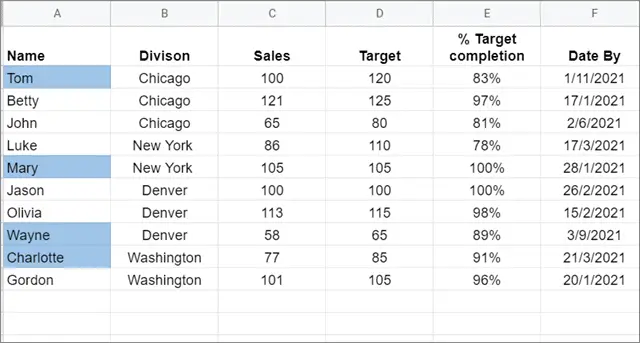
You can easily see that the four names Tom, Mary, Wayne, and Charlotte have been highlighted in the Original Datasheet after referencing them from the Data List spreadsheet.

Conclusion

Conditional formatting is used only when users need to specify data and make it stand out in a large datasheet. Doing so helps with easy navigation throughout the Google spreadsheet and quickly analyzes the specific parameters you are looking for. It also serves as a great way to track goals, giving you visual indications of your progress against particular metrics.

Make sure you select the proper range of cells to highlight while doing conditional formatting in Google Sheets; if mistaken, you might erroneously refer to the erroneous data. You can choose any of the above Google Sheets conditional formatting rules to highlight your data as you wish.