How To Highlight Duplicates In Google Sheets

If you have worked on MS Excel or Google Sheets, you must have encountered instances where you had to weed out duplicates from a datasheet. But, before deleting them, you need to find duplicates in Google Sheets. Hence, it is essential to know how to highlight duplicates in Google Sheets.  

By highlighting duplicates, you can ensure you don’t make any mistake in deleting an original term that has appeared only once in the sheet data. There are multiple ways to highlight data and delete duplicate records and a few sound alternatives to avoid using the highlighting methods. If you don’t want the duplicates, you can also check how to delete duplicates in Google Sheets.

Learn How To Highlight Duplicates In Google Sheets

Google Sheets beginners can turn to the conditional formatting feature to highlight data in a dataset. That being said, let’s take a glance at how to make the duplicates stand out in a document to avoid confusion.

Now that you know the essential steps to identify and highlight duplicates, let us check out the various ways you can do so.

1. How To Highlight Duplicates In A Single Column

First and foremost, let’s look at how we can find out the duplicates in a single column using conditional formatting tools.

Select The Cell Range

Open the Google Sheets document and select the cell range in the entire column. Make sure you don’t select the header row while selecting the column.

Open Conditional Formatting

Now, right-click on the selected column range and choose the conditional formatting option from the drop-down menu. You can also open the conditional formatting sidebar from the Format menu.

Add The Formatting Rule

Now, click on ‘+Add a rule’ to add a new conditional formatting rule.

Set “Format cells if…” to “Custom formula is” and enter the formula given below.

=countif($A$2:$A$10,A2)>1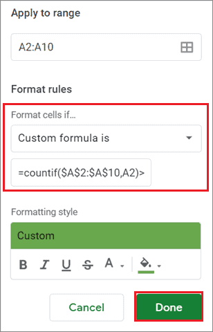

View The Result

Google Sheets will now highlight all the duplicates in your dataset. Also, Google Sheets will mark all the instances of duplicate terms in the selected dataset.

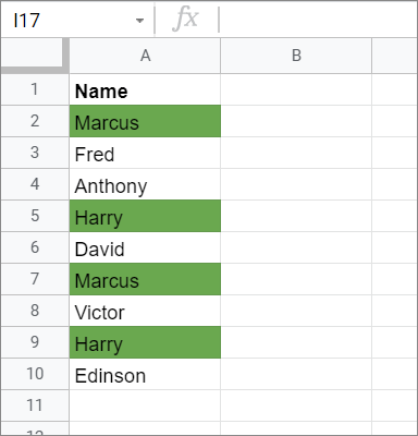
The COUNTIF function is used to count the number of times a text string occurs in the document. If the value is more than 1, the text string is highlighted.

2. Highlight Duplicate Rows In Sheets

We just saw how to highlight duplicates in Google Sheets in columns. Now, let’s see how we can do the same for a duplicate row.

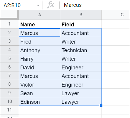
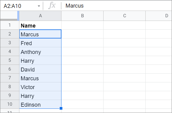
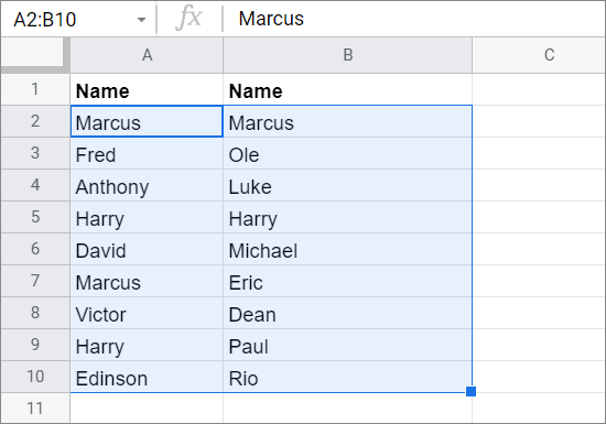
Select The Column Range

First and foremost, select the range of cells in Google Sheets. For this example, we have selected A2:B10 as the range in this sample sheet.

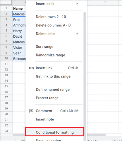
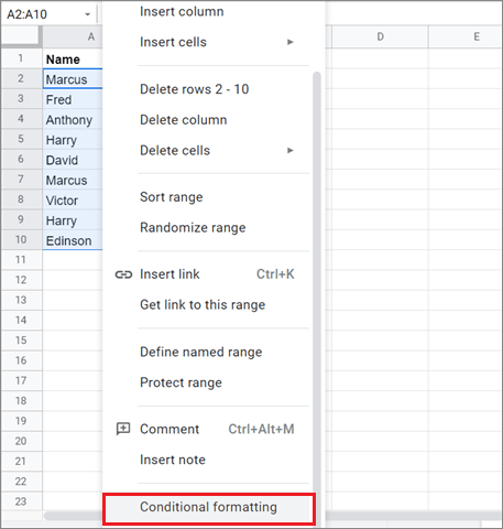
Open Conditional Formatting

Now, right-click on the selected range and choose Conditional formatting from the context menu.

Set The Preferences

In the right sidebar, choose ‘Custom formula is’ in the ‘Format cells if’ field. Enter the formula given below in the formula box and press on Done.

=countif($A$2:$A$10,$A2)>1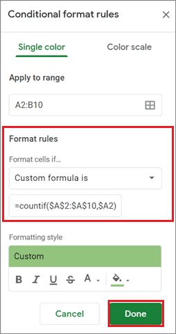

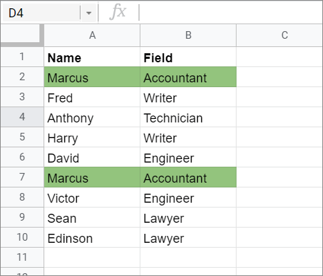
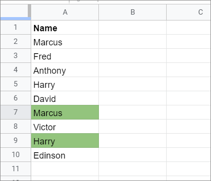
Check The Result

See the result after finalizing the conditional format rules.

3. How To Highlight Duplicate Instances Only

Now you know the basics of how to highlight duplicates in Google Sheets. But, what if some asked to highlight only the duplicates and not the original entries for a particular term? Let’s see how we can do that.

Select The Cell Range

First and foremost, select the range of cells. Here, we have chosen the cells from A2 to A10.

Open Conditional Formatting

Right-click on the cell range and select Conditional formatting from the list.

Enter The Formula

Now, enter the highlight cells rule given below in the blank case.

=countif($A$2:$A2,A2)>1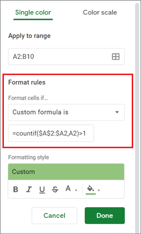

Check The Final Result

Press the Done button and view the result.

4. Create A Unique Cells List

If you don’t wish to highlight a duplicate cell and work with unique value cells, you can use the UNIQUE function in such cases.

Determine The Cell Range

To highlight duplicates in Google Sheets, determine the cell range over which you want to use the function. Here, the cell range is A2:A10.

Enter The UNIQUE Function

Now, enter the UNIQUE function in a cell in column B.

=unique(A2:A10)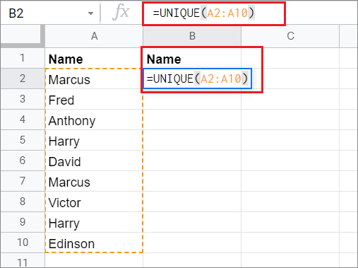

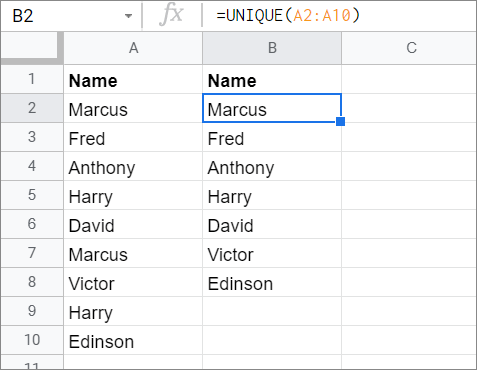
View The Result

Press the Enter key to view the result. You can see that the unique list is created in the column where you entered the function.

5. Eliminate Whitespace To Avoid Confusion

It is normal to have blank space in the cells when we store data in Google Sheets. However, if you enter similar terms in two cells but the amount of whitespace in both cells differs, Google Sheets might not count the cells as duplicates.

So, it’s necessary to trim down the white space to make sure Google Sheets doesn’t get confused.

Select The Range Of Cells

To begin with, select the data range in Google Sheets. Here, we have chosen A2:B10.

Trim The White Space

Now, click on the Data tab in the menu bar and select Trim Whitespace from the drop-down menu.

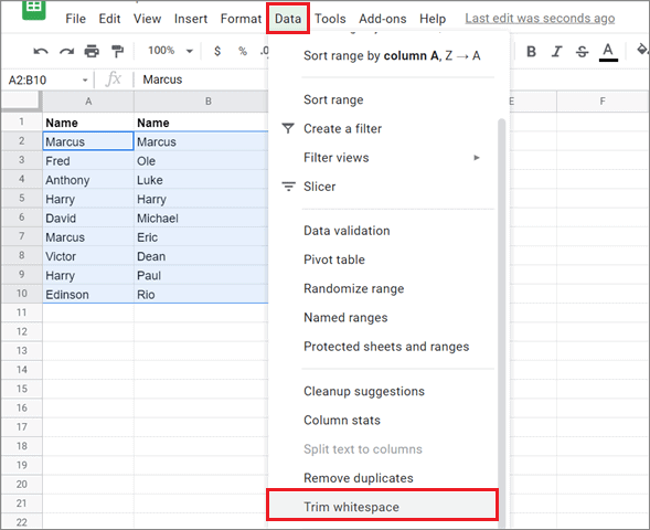
Now, the dataset won’t look any different, but it is ready for evaluation and analysis.

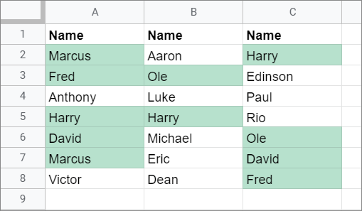
6. Highlight Duplicate Cells In Multiple Columns

We have already seen how you can highlight duplicates in Google Sheets in multiple rows. Now, let’s see how we can do the same for columns.

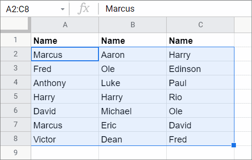
Select The Cells

First and foremost, select the cell range in a datasheet. Here, we have selected A2:C8.

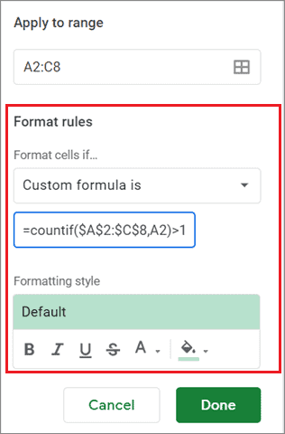
Open The Conditional Formatting Sidebar And Enter The Formula

Next, open the conditional formatting sidebar and enter the COUNTIF formula given below.

=COUNTIF($A$2:$C$8,A2)>1

Click on Done after you enter the function and other customization options.

Check The Result

You can see how the duplicate terms in multiple columns are highlighted by a color in the image given below.

That’s all about how to highlight duplicates in a Google spreadsheet.

Conclusion

Duplicate values can cause data errors in a large spreadsheet, and hence, weeding them out is an essential task. If you are working on sensitive and complex datasets, you can highlight duplicates in Google Sheets and decide to take necessary action later.

Users can either highlight data manually or use a conditional formatting style in a Google Sheets spreadsheet to ease their burden. Assigning a color to duplicate values helps in proper sorting and readability. It also makes sure we don’t delete a unique term erroneously. The action to be taken on the duplicate data depends on the user’s needs and requirements.