8 Ways To Use COUNTIF Google Sheets Command For Data Calculations

While working on complex datasheets in Microsoft Excel or Google Sheets, we often come across instances where we need to count the occurrences of a specific text or numeric term based on a particular condition, also known as a criterion. Counting these terms manually is almost impossible if you are working with many rows in the spreadsheet. This is where the COUNTIF Google Sheets function comes to your rescue.

This function allows users to analyze data in a Google spreadsheet by counting terms in specific areas. The basic syntax for the COUNTIF function is given below.

=COUNTIF(range, criterion)

The range argument is the particular number of cells considered for calculation. Criterion is the specific condition that will be applied to the cells. Criterion is always mentioned in double quotation marks. You can also hide the columns in Google Sheets that contain the function results if you don’t want other users to know about those results.

COUNTIF Google Sheets Function: Count Cells In A Snap!

Before using it in a spreadsheet, know that the COUNTIF function supports only one criterion argument; if you wish to apply multiple conditions, you will need to use different functions for that purpose. On that note, let’s have a glance at how to use this function.

If you are working with numerical data on Google Sheets, you can use the COUNTIF function in eight different ways.

8 Ways To Use The COUNTIF Function

You can opt for any of these ways depending on the data you are on. Let’s take a look at the detailed steps and ways with the help of images.

1. How To Use The Basic Google Sheets COUNTIF Function

Let’s look at the fundamental way we can use the COUNTIF Google Sheets function.

1. Select the columns

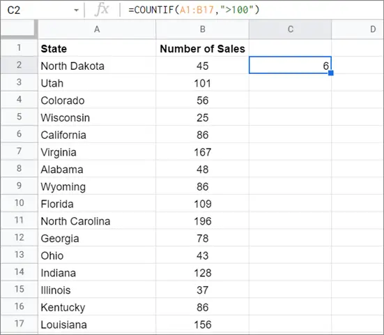
To begin with, select the range argument on which you wish to apply the COUNTIF function. Here, we will select the cell reference A1:B17.

2. Define the condition

In the Sales table given below, we need to find out how many states have made 86 sales. So, the formula for the Google Sheets COUNTIF function is as shown below.

=COUNTIF(A1:B17,"86")

3. View the results

Press the Enter key to view the results. You can see the count of the cells that match the criteria appears in the selected active cell.

2. How To Use The Reverse COUNTIF Function

Now, you can also calculate the results for the exact opposite of the condition we have set. To calculate the number of all states with notched sales figures other than 86, follow this basic formula.

=COUNTIF(A1:B17,"<>86")

3. Use COUNTIF Function With Operators

Now that we know the basics let’s see how we can use the Google Sheets COUNTIF function using a comparison operator. Given below are the five main types of operators that you can use in the COUNTIF function.

1. Greater than: “>”

2. Greater than or equal to: “>=”

3. Less than: “<”

4. Less than or equal to: “=<”

5. Not equal to: “<>”

1. Type the formula

Let’s consider the table from the previous example. We need to extract the number of states where more than 100 sales have been made.

The COUNTIF formula for this condition will be as follows.

=COUNTIF(A1:B17,">100”)

2. View the result

Press the Enter key to obtain the result.

4. How To Use COUNTIF Function With Text

The process of using the COUNTIF Google Sheets function for text terms is similar to what we saw with numeric values.

1. Select the cells

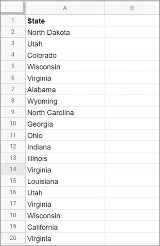
Let’s consider this table to get to know the use of the COUNTIF function. The aim is to find how many times the word ‘Virginia’ has occurred throughout the list. To begin with, select the range argument to apply the function.

Here, the range will be A1:B20.

2. Type the formula

The COUNTIF formula for getting the number count, in this case, will be given below.

=COUNTIF(A1:A20,“Virginia”)

Enter the formula in the cell in which you want to calculate the result.

3. See the cell value of the selected blank cell

Press the Enter key after entering the formula to see the result.

5. How To Use COUNTIF Function With Wildcard Characters

Wildcards help you count any instance of a text; since they aren’t case sensitive, they will count any unique value.

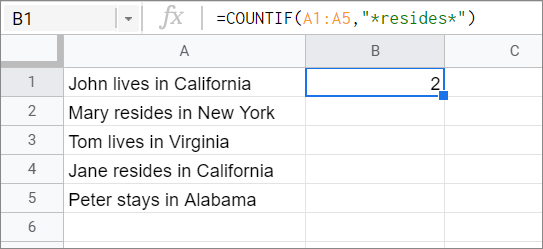
In the table given below, we have to highlight the word ‘resides’ and obtain the count of its occurrence.

1. Select the cell range

Select the range of cells you wish to work on. Here, we have selected the range A1:A5.

2. Enter the formula

Now, enter the COUNTIF formula in a cell. The function for this method is given below.

=COUNTIF(A1:A5,“*resides*”)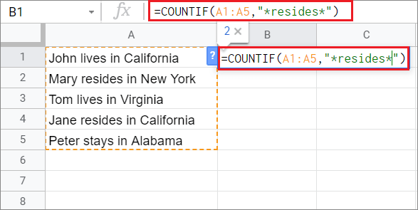

3. View the results

To view the results, press the Enter key. You will see the number of occurrences that appear in the selected cell.

6. Calculating Occurrences At The Start Or End Of A Text String

The two asterisk symbols in the formula allow Google Sheets the flexibility to count the selected term irrespective of the position it appears in the selected range.

For example, in the previous method, we saw that the word ‘resides’ exists in the middle of the text string and not at the start or the end. Hence, we required two wildcards to make Google Sheets count the term.

Now, let’s see how we can calculate the appearances of a term at the start and end of a text string.

1. Calculate occurrences at the start of the string

To begin with, create the COUNTIF Google Sheets function for the table given below. Here, we will calculate the number of times the word ‘California’ occurs at the start of a text string.

The formula for the function is as given below.

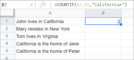
=COUNTIF(A1:A5,“California*”)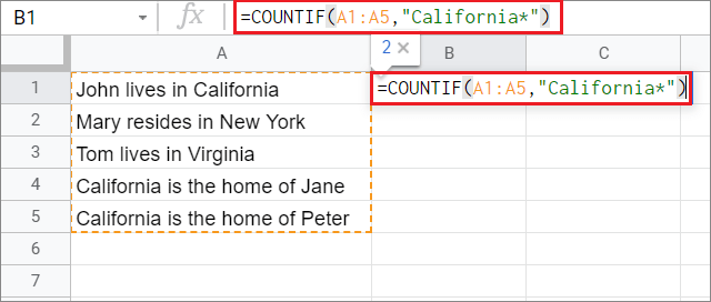

Press the Enter key to see the result. Ideally, Google Sheets should count the term only twice as it appears two times at the beginning of a text string.

2. Calculate the appearances of the term at the end of the string

To calculate the term’s occurrence at the end of the string, we need to place the wildcard character at the start of the term in the function.

This is what the formula will look like:

=COUNTIF(A1:A5,“*California”)

Once you press the Enter key, the result will be shown in the selected cell.

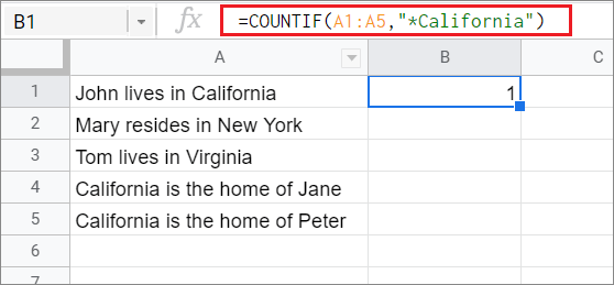
Ideally, the answer should be one because ‘California’ appears only once at the end in a text string.

7. How To Calculate Blank Cells

If you are interested in knowing the number of blank rows in a dataset, you can use the Google Sheets COUNTIF function to your advantage. In fact, this function can also help you obtain the number of non-blank cells in a Google sheet.

1. Select the range cells

To begin with, select the cell range. In the table given below, the selected cell range is A1:B7.

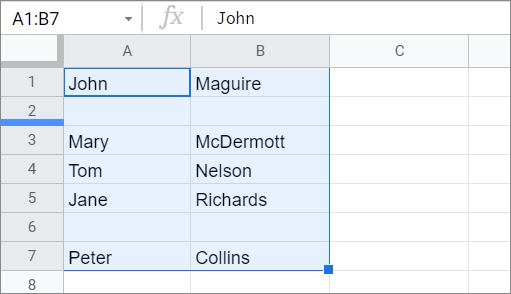
2. Enter the function

Now, enter the formula for calculating blank rows in a spreadsheet. The formula will be as follows:

=COUNTIF(A1:B7,“ ”)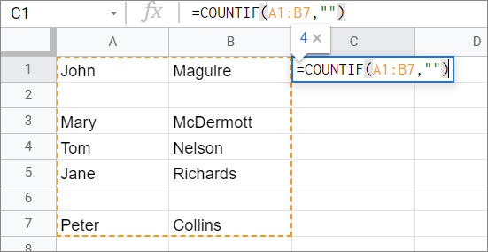

No character in the second string indicates that we are looking out for blank rows.

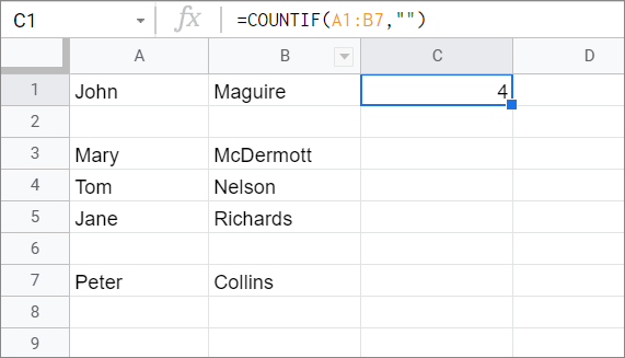
3. View the result

Press the Enter key to view the result. You can see that the number of blank rows appears in the selected.

4. Calculating the non-blank rows

Calculating the number of non-blank rows is a cakewalk; all you need to do is tweak the COUNTIF Google Sheets function as shown below.

=COUNTIF(A1:A7,“<>”)

The symbol “<>” tells Google to count the opposite of what is required.

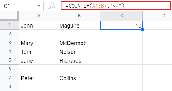
You can see that the appropriate count has appeared in the neighboring column C.

8. How To Use The COUNTIFS Function

If you want to obtain the count for multiple criteria in a single row or columns, you can use the COUNTIFS formula to do so.

The syntax for the COUNTIFS formula is given below.

=COUNTIFS(range1, criterion1, range2, criterion2,...)

1. Select the data range

For this particular example, we will consider the same table we used for the COUNTIF function.

The primary aim is to calculate the number of states with notched sales figures between 100 and 170.

2. Type the function

Now, type the function in a cell in the neighboring column B.

=COUNTIFS(A1:B17,“>=100”,A1:B17,“<=170”)

3. View the results

Press the Enter key and see the results.

The COUNTIFS function is the best choice to go for if you want to obtain results by comparing two or more cell ranges in a Google Sheets spreadsheet. To enhance your sheet further and make it more organized, you can use data validation and conditional formatting in Google Sheets for identifying data quickly.

Conclusion  

Google Sheets provides various functions to make lives easier for users while working on complex and large datasheets. The COUNTIF function helps a user count cells of specific values by exact match and reduces the burden of doing it manually.

The COUNTIF Google Sheets function supports comparison operators and wildcards while executing a set condition over a data range. Also, if you want to match and apply multiple conditions, you need to use the COUNTIFS function.