Google Sheets is used for storing large chunks of numerical data. A standard Google Sheet consists of 26 columns and 1000 rows, which contributes to 26,000 cells in total. However, while working or editing the sheet at times you might want to know we need to know how to hide columns in Google Sheets so that you can read the data properly.
Apart from the hide/unhide feature, users can make graphs, transpose the data, and remove duplicates too. In all, Google Sheets is the best tool not just for storing but also for editing and processing the data.
How To Hide Columns In Google Sheets For Better Data Reading And Analysis
Hiding a column is a better way to get what you want without disrupting the overall formatting of the data. In short, hiding columns or rows as and when necessary helps in efficient comparison of data. Without further ado, let’s have a look at how to hide columns in Google Sheets in different ways.
1. How To Hide Columns In Google Sheets Using Keyboard Shortcuts
Most of us love working on Google Sheets using the keyboard. If you are someone who loves having your fingers glued to the keyboard buttons while entering or formatting the data, there are just a few key combinations that will help you hide a column or a row and unhide it at will.
To hide columns in Google Sheets, use the Ctrl+Alt+0 combination on the keyboard. Doing so will hide the column that you have selected. To hide the rows, press the same combination of keys after selecting the row you want to hide.
2. How To Hide A Single Column And A Row
The process of hiding columns in a Google Sheets document is relatively easy and quick to execute. Users just need to do a few clicks to get the job done.
Select the column that you want to hide by clicking on the column header. Right-click on it and select Hide Column from the drop-down menu that appears.
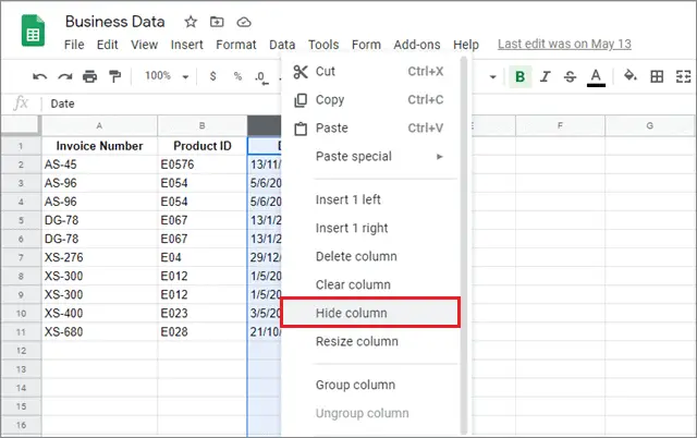
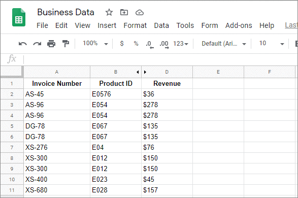
You will see that the column has been temporarily hidden.
Similarly, select the row you want to hide by clicking on the row number. Then, right-click on it and select Hide Row from the drop-down menu.
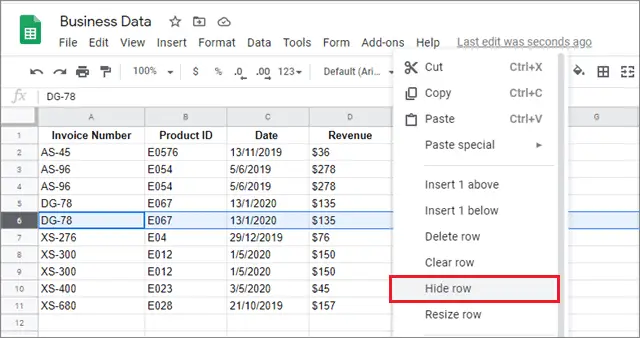
Doing this step will hide the row in question.
Now that we have learned how to hide columns in Google Sheets in the easiest way let’s see how to do the same for multiple rows and columns
3. How To Hide Multiple Rows And Columns
Hiding multiple rows and columns is just as cakewalk as hiding a single row or a column. All we need to do is make sure that the right columns and rows are selected for this step. When it comes to hiding multiple rows and columns, there are two ways of selecting them.
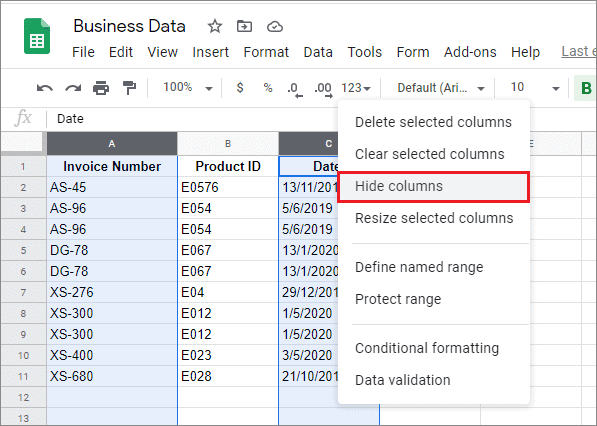
Firstly, if you want to hide columns or rows in contiguous order, say from column A to column C, then you must select them accordingly. Here, we have chosen column A.
To perform a continuous selection, select the column header of the first column. Next, press the Shift key and select the end column. Here, we have considered column D. You will see that all the columns between A and C,i.e., B, will also be selected.
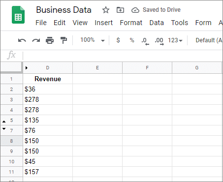
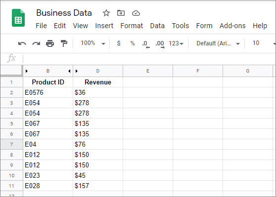
Now, right-click on the selected columns and select the Hide Columns option. You will see that the columns have been hidden successfully.
After carrying out these steps, the columns will be hidden in the Google sheet. The process to hide multiple contiguous rows is the same as shown above.
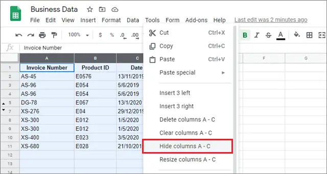
Now, let’s look at another way to hide selected columns. In this example, we have to hide columns in a non-contiguous order. Here, we will select columns A, C, and E.
Select the first column. Then, press the Ctrl key and select the remaining columns manually. In this example, we will select column A first, press the Ctrl key, and then select columns C and E.
Once the columns in question are selected, right-click on any selected column and choose Hide Columns.
Once these steps are carried out, you will see that the selected columns have been hidden in the sheet.
The process to select and hide multiple rows is the same as mentioned for the columns. That’s all about how to hide columns in Google Sheets that are in contiguous and non-contiguous order.
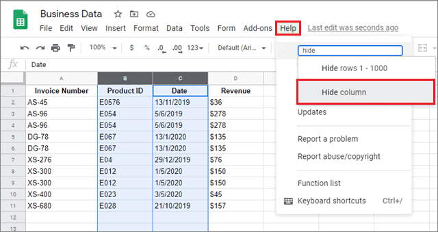
4. How To Hide Columns And Rows Using The Help Menu
An alternative way to understand how to hide columns in Google Sheets is by using the Help menu. Users can easily select the rows and columns and use the Help menu to hide them.
To begin with, select single or multiple rows or columns that you want to hide. Then, click on the Help option in the menu bar and type ‘hide’ in the search bar.
Once you type hide, you will see options for hiding the rows or columns that you have selected. Select Hide row or column as per your selection.
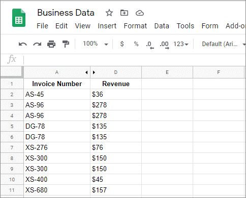
You will see that the row or column in question has been hidden by Google Sheets.
Users can use the Help menu method or the usual method to hide rows in Google Sheets; in the end, it’s all a matter of choice.
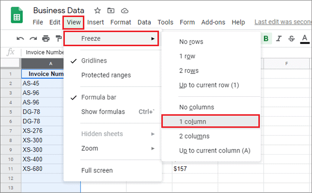
5. How To Freeze Rows And Columns
If you want to lock specific rows or columns instead of hiding them, you can go for the Freeze option. This feature comes extremely handy when you are editing or reading heavy datasheets.
Select a column or a row that you want to freeze. You can also select multiple rows or columns as per the requirements.
Next, click on the View tab and select the Freeze option from the drop-down list. Now, you can choose to freeze the number of rows and columns.
You will see a grey border next to the frozen column. This border acts as the line of differentiation between your frozen and unfrozen columns.
Using the Freeze option will help you to refer to the rows or columns while scrolling through the spreadsheet.
6. How to Hide Columns And Rows In Google Sheets On Mobile
If you don’t have a desktop PC, there’s no need to worry. You can also use a mobile device and learn how to hide columns in Google Sheets.
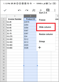
To start with, open the Google Sheets app on your Android or iOS device. Then, select the rows or columns to hide and tap on the shaded area. You will see a menu with options.
If you have an iOS device, tap on the arrow at the right side of the options. Repeat this until you see a Hide option. If you are using an Android device, you can see the menu options by selecting the three vertical dots.
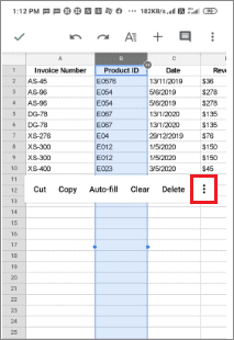
Next, select Hide Row or Column as per the selection. You will see that your selected row or column has been deleted.
Even if you have both a smartphone and a PC, we would recommend working on the latter for a better user experience. Doing such things on a smartphone should ideally be done if and when you don’t have a desktop PC.
How To Unhide Rows And Columns
Now that you have learned how to hide cells in Google Sheets let’s look at how to undo the action and easily unhide columns, rows, and cells. It’s just a one-click process.
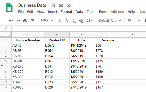
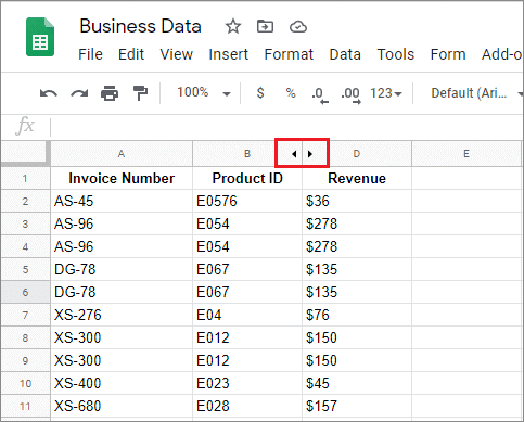
Once you have hidden a column, you will see two arrows pointing in opposite directions on the columns adjacent to the hidden column. Just click on any of the arrows to unhide the column.
That’s all about how to hide columns in Google Sheets. Now you can easily comprehend data easily by making the overall appearance more convenient for reading.
Conclusion
Hiding rows and columns is one of the most important aspects to learn for individuals who have to process, read, and comprehend huge chunks of data daily. When it comes to working on heavy datasheets, users need to compare specific columns or rows with each other frequently. If the distance between these columns and rows is too much, it can be irritating at times to read the data, apart from raising possibilities for errors.
Once you learn how to hide columns in Google Sheets, you can easily read this data without having to do too much scrolling in the datasheet. If your work involves a frequent comparison of rows and columns in a sheet, make it mandatory for yourself to learn how to use this feature. The overall process of hiding a column and row and then unhiding it again is a cakewalk.
Related: How to Use Google Sheets Spell Check To Ensure Error-Free Content


