How To Calculate Days Between Two Dates In Google Sheets

Many people work with dates in MS Excel and Google spreadsheets on several occasions. When it comes to counting days between two given dates, that task can be bewildering and challenging to complete manually. If you often find yourself in a situation where you need to find the number of days, you need to know how to calculate days between two dates in Google sheets.

As easy as it seems, calculating the number of days isn’t possible by simply using a subtraction formula. There are three different functions you can use in these circumstances – DAYS, DATEDIF, and NETWORKDAYS. All three offer a unique way to calculate days between two dates. You can use conditional formatting in Google Sheets to highlight the workday and weekends for ensuring better readability.  If you need to calculate results for multiple pairs of dates in one go, you can use the fill-down method in Google Sheets. 

How To Calculate Days Between Two Dates In Google Sheets

You can count the number of days using the DAYS and DATEDIF formula functions if you don’t mind calculating Saturdays and Sundays occurring between the given dates. However, if you wish to exclude these two days and only count the week days, the NETWORKDAYS formula can help you in this case.

Now that we know the basic steps let’s get into the details with images.

How To Use The Google Sheets Days Between Dates Function

The DAYS function is the easiest to use amongst the lot, provided you aren’t worried about excluding weekends or holiday dates. The standard syntax for this function is given below.

=DAYS(end_date, start_date)

Here, the string ‘date2’ is the end date and ‘date1’ is the start date. The date format is DD/MM/YYYY; you can change the date format as per your preferences using the Format menu.

Since the DAYS function uses a simple subtract function, always remember to put the end date first in the function and the start date after it; doing the opposite would result in a negative answer.

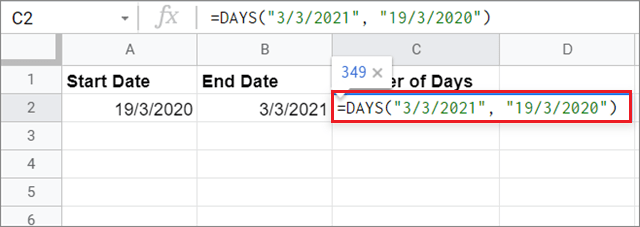
1. Enter The Function

Once you select the sell, create the equation by putting the required dates in the given function.

Here, we have taken dates 19/3/2020 and 3/3/2021.

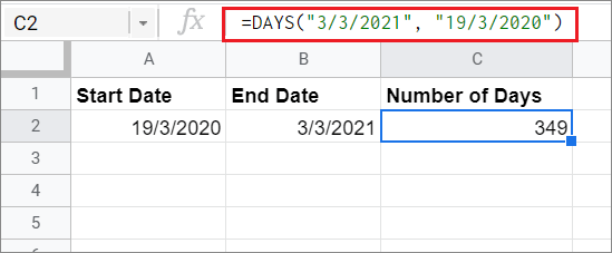
2. View The Result

Press the Enter key to obtain the results.

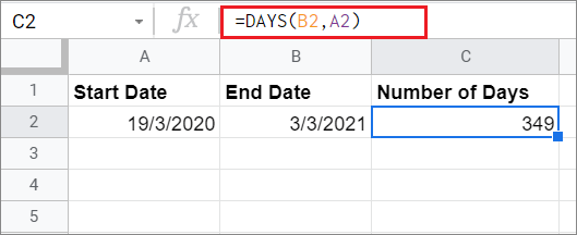
An Alternative Way Of Referencing

If you don’t want to enter the dates in the function, cell referencing is another way to let the Google sheet know the dates you wish to consider in the equation.

Just take a look at this example. Here, B2 and A2 are the cell references of the two dates we have considered for this equation. Just press the Enter key to get the results in the selected cell after you form the equation correctly.

How To Use The DATEDIF Function

The DATEDIF function works like the DAYS function, albeit with two differences.

In this function, you don’t need to add the end date first in the function, like the way you did in the DAYS function. Also, the DATEDIF function helps you gain a count of months and years along with the number of days.

The syntax for the DATEDIF function is given below.

=DATEDIF(“start_date”, “end_date”, “D”)

‘D’ is the unit that denotes the number of days in the equation.

If you wish to use the cell references instead of entering the dates, you don’t need to enter the double quotes over the cell references that indicate the dates. So, the syntax will be as given below.

=DATEDIF(A2,B2,”D”)

1. Formulate The Equation

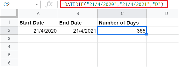
To begin with, create the equation and enter it in the selected cell. Here, we have entered the dates in the equation as given below.

=DATEDIF("21/4/2020","21/4/2021","D")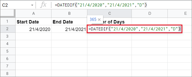

2. View The Result

Press the Enter key to obtain the days between two dates  in Google sheets in the selected cell.

Calculate Month Number

To count the Month number, you just need to make a tiny tweak in the function. Insert ‘M’ in the place of ‘D’ in the formula and press the Enter key to get the number of months between the given dates.

You can change the unit according to your preferences. The accepted units are given below.

Y: the number of whole years between the start date and end date

M: the number of whole months between the start date and end date

D: the number of days between the start date and end date

MD: the number of days between the start date and end date after subtracting whole months

YM: the number of whole months between the start date and end date after subtracting whole years

YD: the number of days between the start date and end date, assuming start date and end date are not more than one year apart.

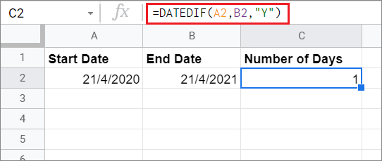
An Alternative Way Of Referencing

Like we did with the DAYS function, you can represent the dates by entering their cell references in the formula.

Here, we have calculated the number of years between the given dates by using cell referencing.

How To Use The NETWORKDAYS Function

Unlike the previous two functions, the NETWORKDAYS function allows a user to consider only business days in the calculation. It assumes Saturdays and Sundays as weekend days and excludes them from the calculation.

The syntax for the NETWORKDAYS function is similar to that of the DATEDIF function; the only change you need to do is replace the Unit with public holidays at the end.

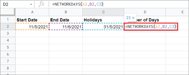
=NETWORKDAYS(start_date, end_date, [holidays]) 

1. Enter The Formula

To begin with, enter the given formula in the selected Google spreadsheet cell to obtain the days between two dates  in Google sheets.

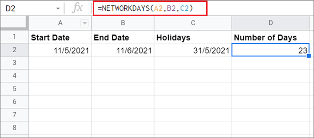
2. View The Result

Press the Enter key to calculate the result. You will get the number of days, excluding the weekend days and the holiday dates defined in the formula.

In this method, we saw how to use the NETWORKDAYS function using cell referencing. You can also use a nested DATE function to represent this function; the syntax is given below.

=NETWORKDAYS(DATE(YYYY,MM,DD),DATE(YYYY,MM,DD))

However, we recommend using cell referencing to avoid creating a lengthy formula so that you can calculate results quickly.

How To Use The DAYS360 Function

If you frequently use a Google sheet for storing financial data and doing interest rate calculations, the DAYS360 function has especially been designed to help your cause.

This function helps spreadsheet users in calculating the date difference in a 360-day year. The 360-day year is primarily used in financial spreadsheets for calculations.

The syntax for the function is given below.

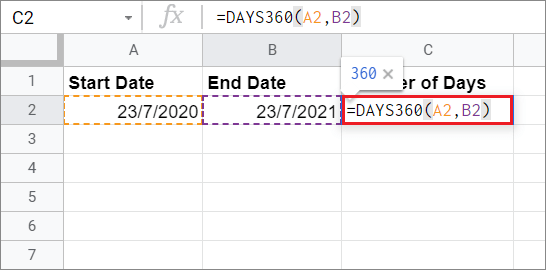
=DAYS360(start_date, end_date, [method])

[method] indicates the day calculate method that should be considered while calculating the number of days. This data value is optional to use and 0 by default.

1. Formulate The Equation

To begin with, enter the formula for the DAYS360 function as shown in the image below.

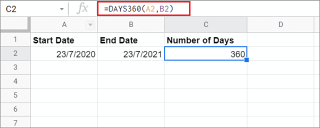
2. View The Result

Press the Enter key to obtain the cell value.

You can use the nested DATE function to represent the DAYS360 function, similar to what we saw in the NETWORKDAYS method. However, using cell reference is a better choice to avoid the detour and calculate results quickly.

How To Use The NETWORKDAYS.INTL Function

The NETWORKDAYS function considers Saturdays and Sundays as weekends while doing calculations. However, what if your off-days are different? This is where the NETWORKDAYS.INTL function comes into play.

This function allows users to consider any single day or two consecutive days to consider as weekends. So, if you have off-days on Thursday and Friday, you can use this function to calculate the days between two dates  in Google sheets.

The INTL stands for ‘International’; this function also allows you to specify your weekends as per your preferences.

The syntax for the NETWORKDAYS.INTL function is as given below.

=NETWORKDAYS.INTL(start_date, end_date, [weekend], [holidays])

1. Formulate The Equation

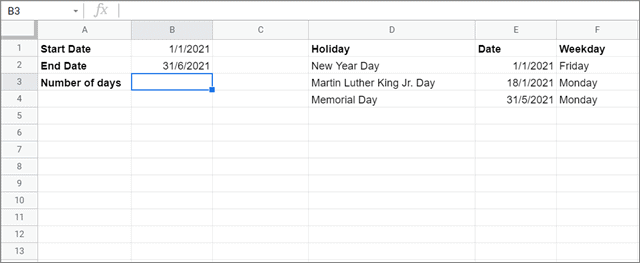
Let’s take this holiday table to understand this equation. Here, we have to exclude all the public holidays and weekends in the given time period and calculate the working day total between dates. In this case, let’s consider your weekends are Wednesdays and Thursdays.

So, the formula for this condition will be as given below.

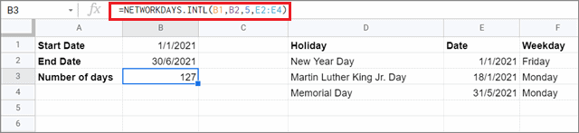
=NETWORKDAYS.INTL(B1, B2, 5, E2:E4)

Let’s specify each argument.

B1 – start date

B2 – end date

5 – the argument that specifies weekends

E2:E4 – data range that considers the holidays

Now, why did we consider the number 5 for specifying the weekends? Because that’s how the code for this function works. The code table is given below.

Code	Days
1	Saturday and Sunday are weekends
2	Sunday and Monday are weekends
3	Monday and Tuesday are weekends
4	Tuesday and Wednesday are weekends
5	Wednesday and Thursday are weekends
6	Thursday and Friday are weekends
7	Friday and Saturday are weekends
11	Sunday is the only weekend day
12	Monday is the only weekend day
13	Tuesday is the only weekend day
14	Wednesday is the only weekend day
15	Thursday is the only weekend day
16	Friday is the only weekend day
17	Saturday is the only weekend day

Users can select any weekend as per their choice using the codes given in this table in the function.

2. View The End Result

Once you have entered the formula in the column cell, press the Enter key to calculate the result.

In this manner, you can use the NETWORKDAYS.INTL function to calculate days between two dates  in Google sheets.

Conclusion

We have seen how the DAYS, DATEDIF, and NETWORKDAYS functions can help us calculate days between two dates in Google sheets. These functions can help you get the number of days in a matter of seconds, provided you enter the functions correctly. One important note to remember is that these functions are based on the US time zone. So, if you live outside the US, you can change the local date and time using the Format menu in a Google sheet.

Before using the functions in Sheets or Microsoft Excel, make sure you determine whether you want to consider the weekend days while calculating days between two given dates. Doing so will help you choose the correct function to work within a Google sheet.