Google Sheets is probably the best tool to go for if you want to store numerical and statistical data. When it comes to statistics, many calculations are involved that require complex formulas. Add the fact that when you apply a formula to one entry, you also need to use the same for all entries in a sheet. That’s when the Google Sheets fill down method comes into play.
Users can easily apply one formula to all the entries in a spreadsheet using this method. Thanks to the convenience it offers, users can complete their calculations at a faster speed. This method also guarantees the accuracy, so you need not worry about rechecking your data for any errors. But at times, users might want to know how to hide columns in Google Sheets so that they can read the data properly.
Top 8 Google Sheets Fill Down Methods To Save Time
There are various methods for doing Google Sheets fill down with formulas. Using this method saves users the time and the need to enter the formulas repetitively. Without further ado, let’s look into these methods and which is the most convenient method for us.
1. How To Fill Down In Google Sheets Using the Fill Handle
The best and the easiest way to fill down Google sheet formulas to every entry in a spreadsheet is by doing the drag-and-drop method. This method requires you to enter your formula only once and then drag it down to the entry up to which you want it to be applied.
First, open the Google Sheets document and select the cell in which a formula has been created. You can use the arrow keys to navigate in the spreadsheet.
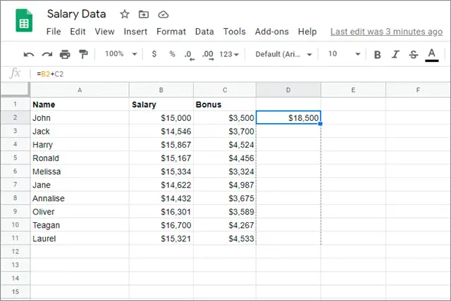
Now, move your cursor to the bottom right part of the selection. You will notice a small blue box here. This square is known as the fill handle. The moment you place your cursor on that fill handle, it will turn into a small black plus sign.
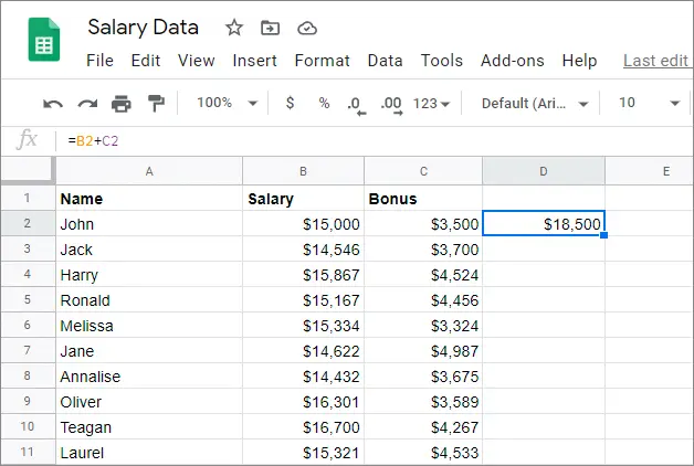
Now, left-click on that fill handle and drag it down to the cell up to which you want the formula to be applied.
After the Google Sheets fill down is done, you will see that the formula has been applied to all the selected cells, and your calculations have been completed.
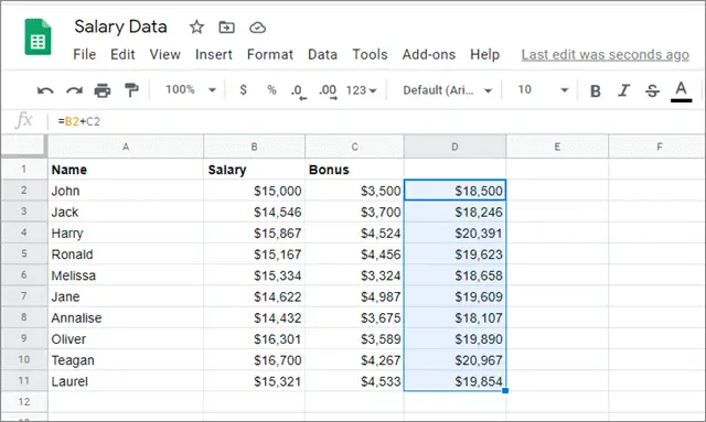
Using the drag-and-drop method saves time and offers convenience compared to all the other techniques mentioned in this article.
2. How To Fill An Entire Column Using An Array Formula
Array Google Sheets formulas also ensure your formulas are applied to a selected number of cells in the blink of an eye. They are relatively easy to execute and do not require any drag-and-drop action for Google Sheets fill down.
First, open the Google spreadsheet from your Drive and select the cell you want to enter a formula. In this example, we will select cell D2.
Now, you have to apply a formula and produce the values in a selected set of cells. For example, we have to produce the addition of cells A2 and B2, and likewise for all the cells mentioned below. To do so, go to the formula bar and type this equation:
=ArrayFormula(A2:A11+B2:B11)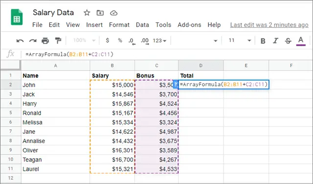
Once you press Enter after entering the above formula, you will get the required value. Then, drag down the formula using the fill handle and fill up the remaining cells wherever needed.
The only drawback of using this formula is that you cannot change the column’s values where the formula has been applied. Since it’s an array, you will need to delete the values in the entire column.
3. How To Fill An Entire Row Using Autofill
Now, let’s look at how we can use the Google Sheets Autofill formula to do the Google Sheets fill down in a single row. This method is also known as the fill right method.
First, open the spreadsheet from your Google Drive in which you want to execute this method.
For instance, we have a series of dates filled in the same row but different columns. We want to fill the same dates in the same locations in the third row.
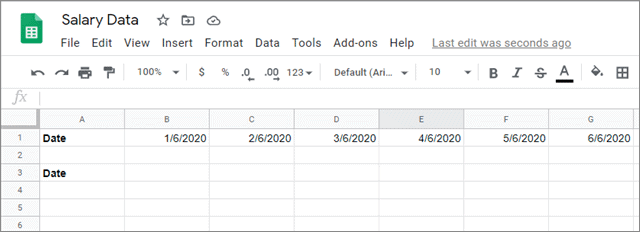
Now, select the cell B3 and enter the formula given below:
=B1This formula will copy and paste the value in cell B1 to cell B3.
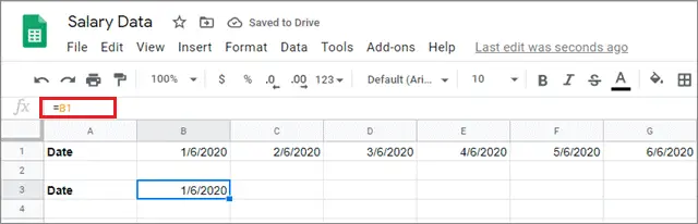
Moving forward, select the cell B3 and click on the fill handle that appears at the bottom-right of the cell and drags it horizontally to the cell up to which you want the formula to be applied.
For example, here, we want the formula used in cell B3 to be used across all the cells up to H3.
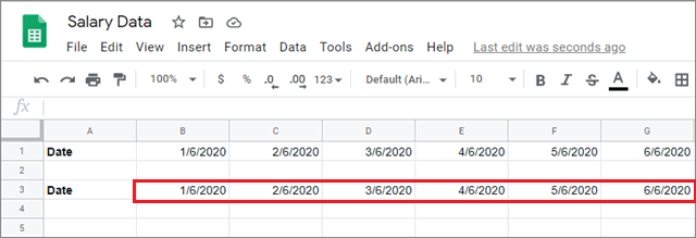
You will see that the formula has been successfully applied to the selected cells after the Google Sheets fill down method has been executed. The same technique can also be applied to columns, only if you have to duplicate one column’s values into another column.
4. How To Fill A Column With Formulas (Combining First Name And Last Name)
Now, we won’t be talking about statistical data.
Suppose if you want to fill the names of employees in an organization, you can use this method to fill the names in columns in a spreadsheet.
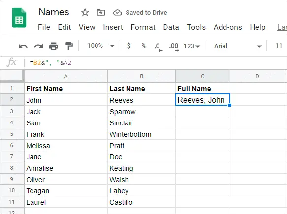
Open your spreadsheet from your Google Drive. Suppose you want to combine the first and the last names of your employees which are entered in different columns, what would you do?
It’s simple. Select a third column in which both the first and last names will be combined. We have the first name in column A and the last name in column B. The combined names will appear in column C.
Now, select cell C2 as the combined name will appear in that cell. Further, type the following formula:
=B2&", "&A2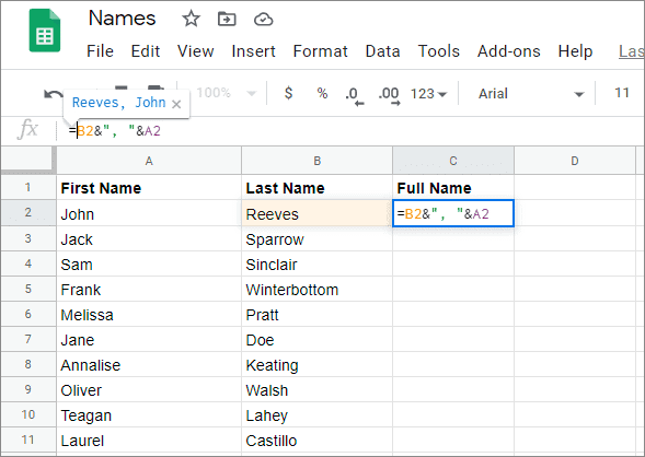
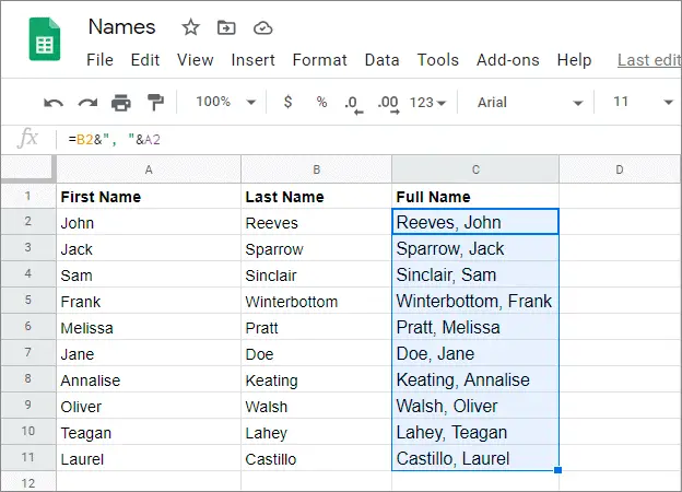
You will now see that the last name and the first name have been combined in a sequence. If you want to change the name’s order, i.e., have the last name following the first name, you will have to make changes accordingly in the formula.
Further, select the cell C2, which has the combined name, click on the fill handle, and drag it down to the cell you want. The values will be automatically filled in the entire column as per your selection.
The process might appear tedious when you are doing it for the first time, but once you get used to the Google Sheets fill down formulas, carrying out these methods is a cakewalk.
5. How To Repeat A Formula (Addition and Multiplication)
Google Sheets also allows users to repeat the formulas while doing the addition and multiplication.
Let’s take a look at how to use the Google Sheets fill down method for repeating formulas.
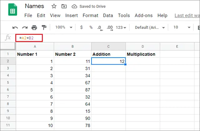
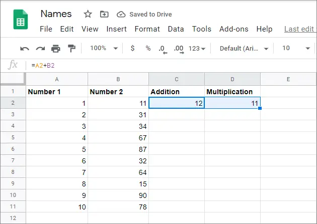
This method involves working in 4 columns. In our case, these columns are A, B, C, and D. Columns A and B contain values, while columns C and D will hold the additions and multiplications of A and B, respectively. We will fill both columns C and D simultaneously in this method.
To begin with, enter these formulas in the two cells C2 and D2, respectively.
=A2+B2 is entered into cell C2
=A2*B2 is entered into cell D2
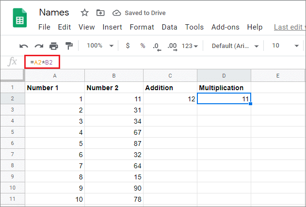
Once you press Enter for both the formulas, the values will show up in the respective cells.
Now, select the two cells C2 and D2. You will notice that the selection pointer stays put on D2, and the fill handle appears in the bottom-right corner of the pointer.
Click on that fill handle and drag it down to the cell D11, which is our final destination.
You will see that the values have been automatically filled in both the columns simultaneously.
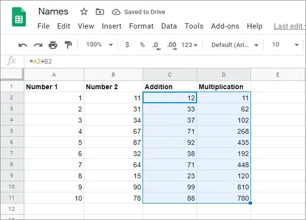
This method allows users to complete calculations in multiple columns simultaneously, meaning users can always complete their calculations within no time.
6. How To Fill Down A Formula In Google Sheets Using IF Function
Google Sheets fill down with the IF functions that can be used when you have to classify entries into certain groups. For example, the IF functions can help teachers sort a group of students into passed and failed groups.
First, open the spreadsheet from your Google Drive containing the students’ names and grades. Suppose column A has names and column B has marks, column C will show whether the student has passed or failed.
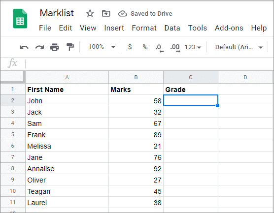
Enter the following formula in cell C2
=IF(B2>40,"Pass","Fail")After you press Enter, the value will appear in the selected cell, i.e., C2.
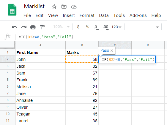
Now, select C2, and use the fill handle at the bottom right corner to apply the formula across a range of cells, in this case, from C2 to C11. The students are then sorted into groups according to the user’s requirements.
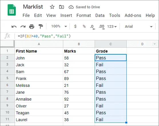
The IF function will save users the trouble of sorting out their entries manually by carrying out that process in the blink of an eye.
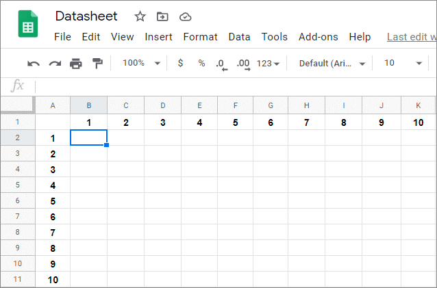
7. How To Autofill A Table Of Formulas In Google Sheets
You can also use autofill to fill an entire table with formulas, where the formulas will be copied in both the horizontal and vertical directions at the same time.
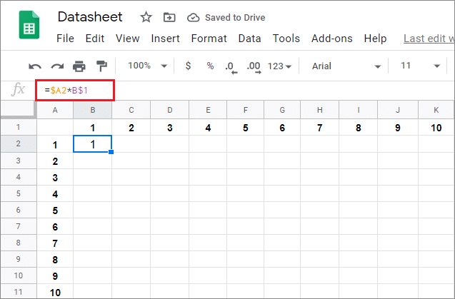
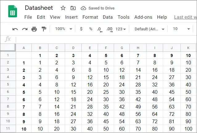
To begin with, open the spreadsheet from your Drive. Now, this sheet is different in contrast to other sheets. Here, we have a series of numbers incrementing in series across rows and down the columns. Our aim is to copy our initial formula entered into cell B2 into the whole table of cells so that each of the formulas multiplies the values displayed on the top left side of each column or a row.
You will also notice the use of the dollar ($) sign in the formula. This sign is used to lock an entire column or a row when cells and formulas are copied. It is also known as an absolute reference, meaning it helps the formula in referring to values from a fixed column or a row while doing calculations.
The $ sign has been implemented in such a way that when the formulas are copied to the right, they will continue referring to numbers in column A. However, they will also adjust vertically as the numbers in column A increment.
Now, enter the formula given below in cell B2. This formula will then be copied across the entire range of B2:K11.
=$A2*B$1After Pressing Enter, you will get the value in B2.
Select B2 and drag it across the entire range. The formula will be copied and executed in all the selected cells.
Auto-filling a table might appear to be an uphill task for beginners, but it’s just a matter of time before you get used to it.
8. How To Use Google Sheets Fill Down On Mobile
For all those who need to execute the fill down Google Sheets method urgently but do not have a laptop or computer at hand, they can do the same on their smartphones as well.
First and foremost, open Google Sheets on your smartphone. Then, open the spreadsheet in which you wish to execute the fill down method. Now, select a cell in which you want the value to appear after the method is executed. This is the cell where you have to enter a formula and press Enter.
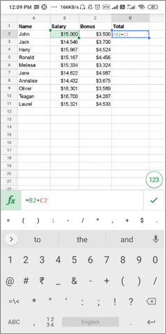
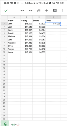
After the value appears in the formula, select that cell. In our case, we will select the cell C2.
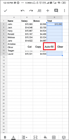
Now, you will see a tiny circle in the bottom right corner. This is how the fill handle looks on a smartphone. Use the fill handle to drag the pointer down cell C11.
Once you have executed the Google Sheets fill down method, you will see a menu containing four options.
Select ‘Autofill’ from the menu.
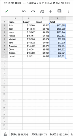
The values will be generated in the selected cells.
All the methods executed above can be carried out on a smartphone as well. However, we recommend using a laptop or a PC for a better view, convenience, and ease of operation.
Conclusion
Google Sheets is one of the most preferred tools for storing numerical or statistical data. It helps users in carrying out simple mathematical calculations with pinpoint accuracy. As a result, you need not worry about any errors if you are using Google Sheets for doing calculations.
When it comes to number-crunching in a broad datasheet where a formula needs to be applied to various cells, you can use the Google Sheets fill down method for ease of calculations. There are different types of formulas that can help you carry out several types of calculations. Users also use Google Sheets drop-down to validate the data.
While the drag-and-drop method of filling down formulas remains the same, it all depends on the types of formulas that are being used for various purposes. The choice of formulas depends on the type of data you are editing.
(Updated on 7th January 2021)


