Both Microsoft Excel and Google Sheets offer various functions that you can use on your datasheets for multiple purposes. One of the most common functions in use is the Google Sheets IF statement, which allows a user to perform logical function tests based on specific conditions.
Using the IF statement, you can choose to take certain actions on specific parts of your datasheet if they satisfy a predefined condition in a Google sheet or an Excel spreadsheet. This function compares data in the selected range with the given condition and then produces the required result. If you have a more extensive datasheet, you can use the COUNTIF function to determine the number of positive results.
You can also use the Google Sheets fill-down method to apply the function and get multiple results in one go.
How To Use Google Sheets IF Function To Get Accurate Results
The IF statement can also be used with various other functions to obtain results in different datasets. That being said, let’s take a glance at how to perform this function by seeing a few simple examples.
3 Steps To Use Google Sheets IF Statement
1. Open the Google Sheets.
2. Select the cell and enter the formula.
3. Press Enter key to view the result.
Now that we know the basics of using the IF function in different scenarios, let’s see how to use Google sheets IF function with details and images.
1. How To Use The Google Sheets IF Function
Before we move on and directly apply the formula, let’s glance at how the IF function syntax looks like.
IF (logical_expression, value_if_true, value_if_false)
Let’s dissect the parts of this function.
1. logical_expression – The expression that has a logical value. For example, TRUE or FALSE.
2. value_if_true – The value that the function will return if the logical test expression is true. The returned value can be a text string, number, or even a function that returns a value.
3. value_if_false – The value the IF function will return if the logical expression is false. The returned value can be a text, number, or even a function that returns a value.
Now, let’s look at how the IF function works.
Enter the formula in the given cell
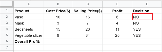
To begin with, here’s a small table template over which we will see how to use the Google Sheets IF function. In this table, we have to decide whether to go ahead and sell a particular product or not.
The condition for selling the product is that the profit should be equal to $10 or more.
Now, the Google Sheets formula for the equation will be given below.
=IF(D2>=10,“YES”,“NO”)
If the numeric values in the entire column D are greater than 10, the function will return YES. If it is less than 10, the function will return NO.
View the result
Press the Enter key to obtain the result. You can drag down the result to get values for the entire range of cells in the given table.
2. How To Use The IF Function With Calculation As A Result
We saw how we could get text results while playing around with numbers in the IF function in the previous method. Now, let’s see how we can obtain calculations as a result.
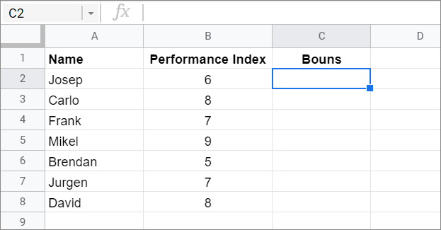
Let’s look at the table given below to understand how the Google Sheets IF function will work in this case.
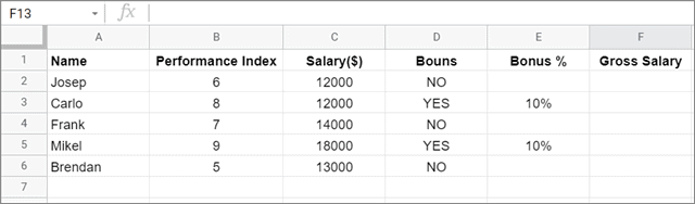
Here, we will award bonuses to employees who have notched a Performance Index of 8 points or above. We will also include the appropriate function that will calculate the total salary, including the bonuses.
Enter the equation
We already know which employees deserve a bonus, so let’s get directly into the formula for calculating the gross salary using the IF statement in Google Sheets.
Enter the given custom function in the formula bar or the blank row in which you want the results.
=IF(D3=”YES”,C3+(C3*D3),C3)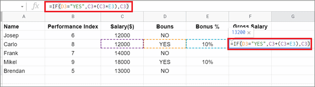
Notice that we have inserted the formula for calculating the gross salary in place of the value_if_true condition.
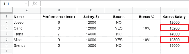
Check the result
Now, press the Enter key to view the results in the selected fields. Based on cell B2 and cell B5, we can see that Carlo and Mikel have earned the bonuses.
3. How To Use The Nested IF Function In Google Sheets
The simplest definition of the nested IF function is ‘using an IF function within another IF function.’ You can nest the IF function with either value_if_true or value_if_false expressions.
Let’s consider the previous worksheet table below to understand the nested function operation. Now, the main aim here is to allot the bonuses as per the Performance Index(column B) using a nested IF function.
We have to satisfy the three conditions given below by using the IF function to obtain the actual result.
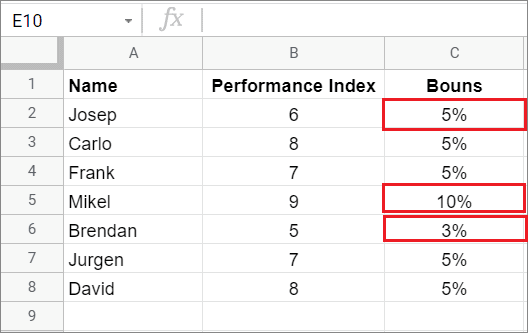
1. Employees with a PI 5 or below will have a 3% bonus
2. Employees with a PI between 6 and 8 will get a 5% bonus
3. Employees with a PI more than 8 will get a 10% bonus
Enter the custom function
To begin with, form the equation for the three conditions. The simple basic is to group any of these two criteria in an IF function. Then, use that IF function to nest another IF function involving the third criteria.
We will use a nested function with the value_if_false expression to obtain results in the blank cells. The custom formula in the single cell C2 will be as given below.
=IF(B2<=5,“3%”,IF(B2<=8,“5%”,“10%”))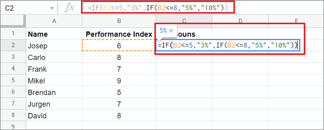
Obtain the result
Press the Enter key to get the result. You can drag the result in C2 to obtain the result based on cell B3 and beyond.
4. How To Use The IF Function With AND Function
You can use the Google Sheets IF function with the AND function when you wish to satisfy multiple conditions in an equation.
Let’s consider this table of football strikers contesting for a place in the national team. Now, the main aim is to select strikers based on two conditions.
1. The number of goals should be 30 or more
2. The strike rate should be 70% or more
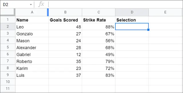
The strikers who satisfy both the conditions mentioned above will earn a place in the national team.
Now, let’s look at how we can solve this issue with the AND function.
Enter the function
To begin with, enter the equation given below.
=IF(AND(B2>=30,C2>=70%),“YES”,“NO”)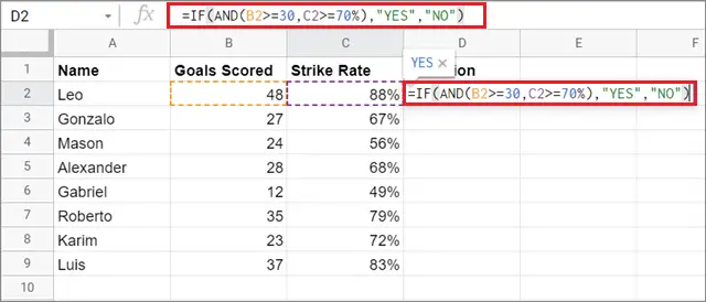
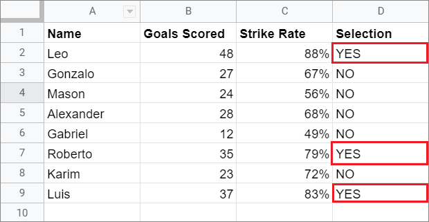
Check the result
Press the Enter key to view the result in the selected fields. You can see that the strikers who satisfy both conditions are selected. You can use conditional formatting in Google Sheets to further highlight the selected candidates to ensure ease of readability.
5. How To Use The IF Function With The OR Function
The OR function works exactly opposite to the AND function. You can use this single formula whenever you want a minimum number of conditions satisfied by many criteria.
Let’s look at this table. The primary aim is to select candidates for a position in a company based on two given conditions.
1. The candidate should have an aptitude score of at least 18 or more.
2. The candidate should score at least 15 or more points in the interview.
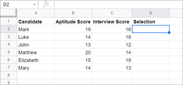
Your primary aim is to highlight candidates who satisfy both or at least one condition to qualify for the next round of tests.
Now, let’s check out how to execute the OR function with the Google Sheets IF function in this case.
Enter the formula
Enter the formula in the given table in the Google Sheet.
=IF(OR(B2>=18,C2>=15,“YES”,“NO”)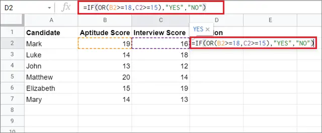
Check the result
Press the Enter key to obtain the result in the selected fields.
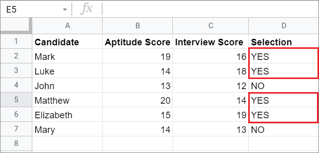
Now, you can see that Mark and Elizabeth satisfied both parameters and were selected for the next round. Similarly, Luke and Matthew satisfied only one of the given conditions and also passed for the next round.
Conclusion
Google Sheets IF statement is widely used for calculations in spreadsheets where you need to compare cell values with certain conditions and then obtain a result. You can perform various numerical and logical tests using the IF statement in a Google Sheets spreadsheet. You can also use the IF function in the Google app.
This function can also be used in tandem with various other functions like AND and OR. You can also use the logical operators shown in this article to set the conditions for comparison with the cell values. A user can apply the IF function for different purposes in different datasheets, so the use of this function depends entirely on the data in which it is being used.


