How To Use SUMIF Function In Google Sheets

Google Sheets and Microsoft Excel spreadsheet users are pretty well-acquainted with formulas and functions for analyzing large data spreadsheets. A few of these Google Sheets functions are pretty simple to comprehend, while many others require some time for proper understanding. SUMIF function in Google Sheets is one such formula you may need to learn if you are just getting started in the world of business and data analytics.

SUMIF Google Sheets function is an amalgamation of the SUM function and the IF statement, respectively. It allows users to summarize data in large spreadsheets by scanning cells that comply with a given condition. Once a matching cell is found, the number corresponding to the cell is included in a group of selected numbers.

How To Use The SUMIF Function In Google Sheets

The Google Sheets SUMIF function is used to add specific numbers that meet a particular condition. Let’s glance at how we can use this function to help our cause in different scenarios.

Now that you know the basics let’s move on to the step-by-step explanation with examples. Before we begin, let’s take a look at the function syntax.

Syntax Of The SUMIF Function

The syntax of the SUMIF function is given below.

=SUMIF(range,condition,[sum_range])

Now, let’s understand the different parts of the function.

Range – the group of cells on which the SUMIF Google Sheets function will be performed.

Condition – the specified criterion that helps in classifying the spreadsheet terms.

[sum_range] – This is an option character. [sum_range] is the range of cells containing values added if its corresponding number in range matches the condition. If this term is not included, then the ‘range’ is assumed as the sum range in the function.

So, now it’s clear that you can use the SUMIF function in two ways: 

1. Without a separate [sum_range]
2. With a separate [sum_range]

Example:

If all three parameters are given in the SUMIF Google Sheets function, it will first check if the first given range satisfies the condition. If it does, the function will consider and include the corresponding cell value in [sum_range] for the final sum calculation.

If the [sum_range] value isn’t specified, the SUMIF function will add only those cell values from the cell references that satisfy the condition.

5 Simple Ways To Use SUMIF in Google Sheets

There are 5 simple ways in which you can use SUMIF in Google Sheets.

1. How To Use The SUMIF Google Sheets Function With Numbers

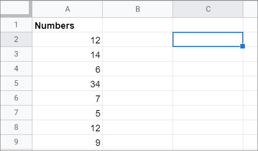
We will consider the sample Google spreadsheet given below and calculate the Google Sheets sum of numbers that are less than or equal to 10. We will calculate the result in cell C2.

Now, let’s see how we can calculate the sum using the SUMIF function.

Enter The Function

Once you select the cell in which you want to obtain the result, enter the SUMIF function.

In our case, the Google Sheets formula will be as given below.

=SUMIF(A2:A9,”<=10”)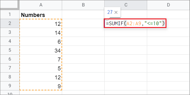

View The Result

Press the Enter key to see the sum data in the spreadsheet.

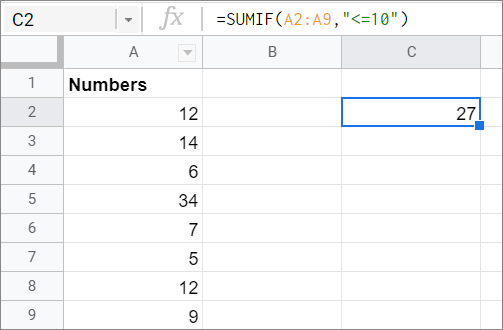
You can see that the numbers complying with the given condition(6, 7, 5, and 9) are considered in the calculations.

2. How To Use The SUMIF Function With Text

Now, let’s look at how to use the SUMIF Google Sheets function with sheets containing a text string.

We will consider the sample sheet given below.

The aim is to calculate the total number of sales made by Monica and obtain the result in cell D2.

Enter The Function

Form the function formula according to the given condition. In our case, the SUMIF formula will look like this.

=SUMIF(A2:A9,"Monica",B2:B9)

View The Result

Press the Enter key to obtain the result in the selected cell.

Now, notice the difference between the two examples. We didn’t need to specify the [sum_range] part in the function in the first example, but we did so in the second.

Here, the SUMIF function first checked which cells from the first range match the condition and then selected the corresponding cell values from the cell reference of the second range, i.e., B2:B9.

It’s important to note that the [sum-range] part is necessary while working with specific text strings in the SUMIF function.

3. How To Use SUMIF With Dates

Now, let’s see how we can use the SUMIF Google Sheets function in spreadsheets containing dates.

Before we move on with the method, it is essential to specify the format of displaying dates in Google Sheets. You can specify that using the Format menu in the menu bar. 

Once you have decided upon the date format, we will use this sample sheet given below to understand the concept.

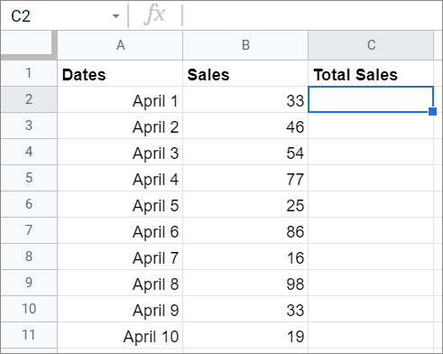
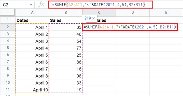
The main aim is to calculate the total number of sales in column B up to April 5 in cell C2.

Enter The Formula

To begin with, formulate the function and enter it in the selected cell. In our case, the formula is given below.

=SUMIF(A2:A11,"<"&DATE(2021,4,5),B2:B11)

Notice the default syntax for the DATE function here is (year, month, day). You have to input the date according to the DATE function syntax.

Also, you need to use the ampersand(&) symbol to concatenate the “<” operator to the DATE function.

View The Result

Once you press the Return key, the answer will show up in the selected cell.

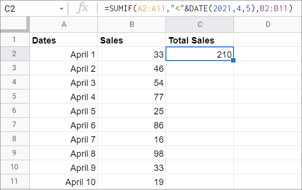
According to the given formula, the SUMIF function has returned the sum of all the sales made before April 5; the values for April 5 are not considered in the function.

If you want the SUMIF function to consider it, change the operator from “<” to “=<” in the equation.

4. How To Use SUMIF With WildCards

You can also use the WildCards with the SUMIF function, although it’s not mandatory to do so.

For this example, we will use this sample sheet given below.

The primary aim is to calculate the quantity of all the products related to a TV. Let’s see how we can do it using this example.

Enter The Formula

To begin with, select the cell, C2 in our case, and enter the SUMIF function as shown below.

=SUMIF(A2:A7,"TV*",B2:B7)

View the result

Now, press the Return key to obtain the results in the selected cell. In this example, the formula considers values from SUMIF cells, B2, B3, and B7, because their corresponding cells in the entire column A have the term ‘TV’ in it.

The asterisk sign ‘*’ is a WildCard character. This single character tells Google Sheets to look for all the cell values containing a specific term in a defined data range. WildCards don’t ask for an exact match, but just the presence of the specified term.

5. How To Use SUMIF Function With Blank And Non-Blank Cells

The SUMIF Google Sheets function can also be used with blank and non-blank cells. Let’s see that with this sample Google sheet given below.

Now here, you have to calculate the sum of only non-blank cells in cell C2.

Enter The SUMIF Formula

Enter the Google Sheets SUMIF formula in the selected cell. It will be as given below.

=SUMIF(A2:A7,"<>",B2:B7)

The logical operator “<>” denotes the non-blank cells.

View The Result

Press the Enter key to view the sum value in the selected cell.

Now, suppose if you want to check the sum for the corresponding cell values of a blank cell, you can use the ” ” instead of the “<>” logical operator.

In this case, the SUMIF function has considered cell values from B3 and B6 because their corresponding cells in column A are blank. Taking a step further, you can also use conditional formatting to mark the cell range that SUMIF has considered in the calculations.

Users also need to know the fact that the SUMIF formula cannot be used within an array formula. You can use the SUMIF formula mostly in a Google Sheets budget spreadsheet where you need to calculate values corresponding to a specific text string.

Conclusion

SUMIF in Google Sheets allows users to calculate the sum of numbers in cells that meet a single criterion, a specific criterion, or multiple conditions. Apart from numbers, it can also be used with data containing text strings and numbers. It also happens to be one of the essential functions for data analysis in Google Sheets.

While using the SUMIF function in Google Sheets, there are specific points to keep in mind if you want to avoid errors. If you want to add numbers that satisfy multiple criteria instead of one, you need to use the SUMIF formula.