When we work in Google Sheets or Google Docs, it is vital to organize data for better comprehension. The reason being we work with many headers and columns while using this tool for data storage. An organized datasheet helps users better understand the figures, which is why we need to know how to merge cells in Google Sheets.
Merging cells isn’t the only way to ensure proper data organization; you can also learn to add bullet points and link cells in Google Sheets. In Google Docs, cells are merged in the tables that are created by the users.
How To Merge Cells In Google Sheets
Suppose you have a datasheet entailing all the quarterly figures for revenue and profits of your business. You can merge the ‘revenue’ and the ‘sales’ columns under the ‘Q1’ header column, and do the same for all the other quarters. Doing this will help you to analyze the data in detail and point out the shortcomings.
So, let’s look at how to merge cells in Google Sheets and also learn how to combine the contents of multiple columns in a single cell.
How To Merge Cells In Google Sheets Using The Format Menu
The easiest way to merge selected cells in Google Sheets is by using the Format Menu. With a few simple clicks, you can easily organize data using the Google Sheets merge cells feature.
To begin with, select the cells you want to merge and go to the Format menu. Then, click on the Merge option and select ‘Merge all.’
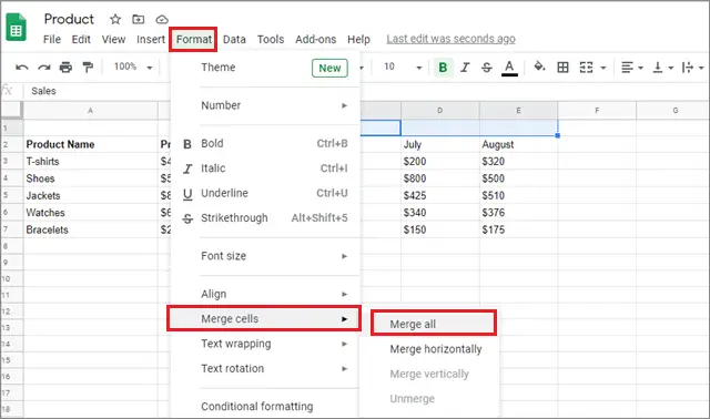
Once you do this, all the selected cells will be merged, as shown in the figure below.
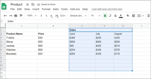
Users need to know that only the content in the left-most cell will be kept intact while merging cells. If there is any content in any other selected cell, Google Sheets will prompt you. That’s the simplest way to learn how to merge cells in Google Sheets.
Variety of Merge Options
1. Merge All
When you select Merge all, all the selected cells are merged into one big cell. To use the merge cell Google Sheets feature, you must choose the cells first.
2. Merge Horizontally
The Merge horizontally option is used to merge cells horizontally. When you select multiple rows and use this option, the columns will be eliminated from your selection.
3. Merge Vertically
When you avail the Merge vertically option, the rows in your selection will be eliminated, and you will get a sizeable vertical cell, which is the result of a combination of multiple vertical cells.
How To Merge Cells Using A Separator
Now that you have learned the basics let’s look at how to combine cells in Google Sheets.
At times, we often deal with data where we require separators to mark the difference between the combined entities. In such cases, you can merge cells in Google Sheets using a dash, comma, or any other character.
Suppose you want to combine the data in columns A and B with a dash acting as a separator. Select a cell in column C and type the following formula to merge horizontally.
=A2&”-“&B
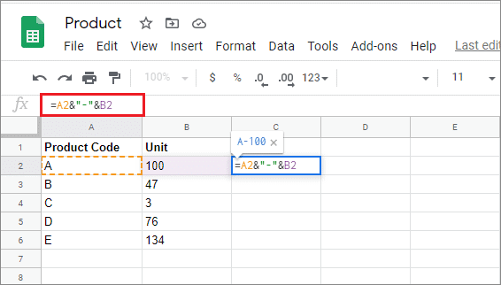
This is how the combined result will look like.
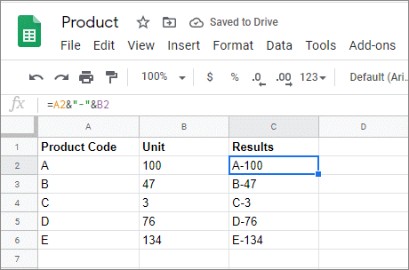
The character ‘&’ is used to combine the two entities with ‘-‘ acting as the separator between them. You can also use the Concatenate function to carry out this task. Enter the following formula.
=CONCATENATE(A2,”-“,B2)
You will have to specify the entities in this formula without using the ampersand.
How To Merge Cells Without Separators
Suppose you want to merge cells A2 and B2. Select a cell in which you want to combine the content in these cells. Enter the following formula:
=A2&B2
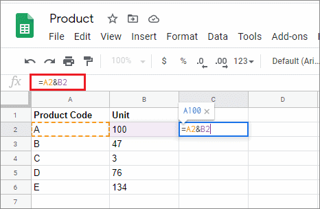
You will see that A2 and B2 have been combined successfully in the selected cell, i.e., C2.
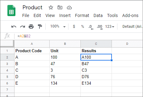
The only difference here is that you have to remove the ‘-‘ separator and enter the remaining formula as it is in the cell.
How To Combine Cells With Separated Line Breaks
Suppose you have a datasheet of addresses of your employees that is split into various columns such as name, street, city, and state, as shown in the figure below.
While learning how to merge cells in Google Sheets, you need to know that line breaks are essential to separate the different parts of an address. You cannot just combine cells and write the entire address in a single line.
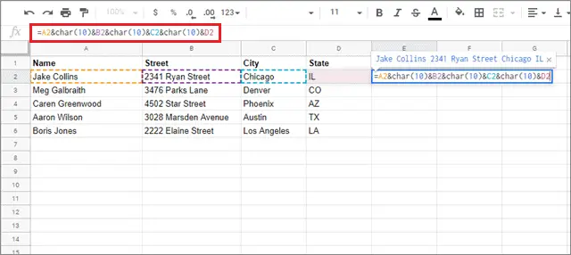
To start with, select a cell in which you want to produce the result. Then, enter the following formula in it and press the Enter key.
=A2&char(10)&B2&char(10)&C2&char(10)&D2
You will see that the line breaks will be applied after each entity in the address.
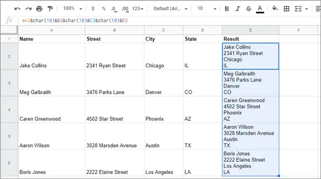
The vital thing to know about here is the CHAR(10) function, which creates the necessary line breaks. Make sure you have the text wrapping function available before you do this step, lest you want the result to spread out of the space of the cell.
How To Combine Text With Percentages
Percentages are essential for measuring many KPIs in business sheets. However, combining text with the percentages can be a real hurdle as Google Sheets doesn’t merge them as they are.
For example, refer to the A and B columns in the following image. You have to combine the text with the percentage in this example and produce the result in a different cell.
Now, using the primary way, you would use the formula =A2&B2 to combine the results. However, the percentage is converted into decimal numbers by using this formula.
To avoid this conversion, you need to tweak the formula a bit.
=A2&” – “&TEXT(B2,”#.00%”)
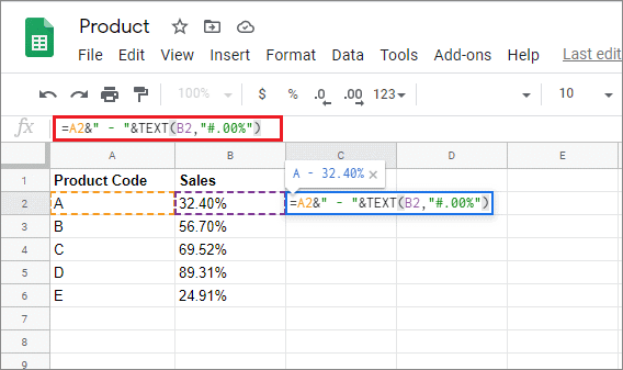
The TEXT function is used to keep the formatting of the cells intact while combining them.
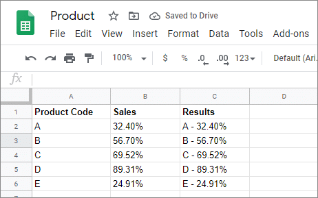
That’s all about how to merge cells in Google Sheets when it comes to combining text and percentages.
How To Unmerge Cells In Google Sheets
Now that we have learned the basics of merging cells in Google Sheets, lear’s learn how to do the opposite. Unmerging the merged cells is nothing but backtracking on the steps you followed to merge them.
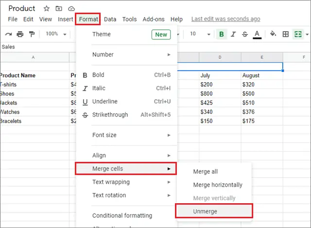
To begin with, click on the Format button in the toolbar and select Merge cells.
Then, click on Unmerge from the drop-down menu.
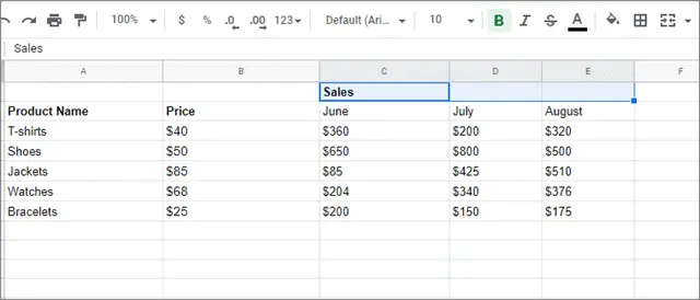
The cells will immediately be unmerged, as shown in the figure.
Merging and unmerging cells is a simple process altogether. If you can learn the formulas mentioned in this article, you can easily carry out the steps and tweak the formatting of cells as per your requirements.
How To Merge Cells On Smartphone
Merging cells on your smartphone is as simple as doing it on a PC or a laptop. With just one tap, you can merge any selected number of cells.
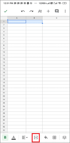
Open the Google Sheets application on your mobile and enter a new spreadsheet. Then, select the cells you want to merge and tap the Merge option, as shown in the figure below.
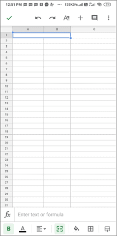
As you will see, the cells get merged immediately.
The mobile version of Google Sheets doesn’t offer enough customization options to merge or combine cells. However, you can combine the selected cells using all the formulas as you do on a desktop.
Conclusion
Google Sheets is one of the most vital tools used for numerical and statistical data storage. While there are multiple ways to ensure proper data organization, the Google Sheet merge cells feature enables better comprehension for analysis of data. This is the very reason why we need to learn how to merge cells in Google Sheets.
Merging cells can be done for different purposes. It is usually done to represent multiple columns under one header column. You can use the merge cells Google Sheets feature in the Format menu. Also, it is possible to describe the results of multiple selected cells in a single cell. Furthermore, cells can be merged either horizontally or vertically. The decision to merge cells in Google Sheets depends upon the user’s needs and requirements; it isn’t a mandatory feature to use.
Related: How To Use Google Sheets Split Text To Columns Feature


