When it comes to storing statistical data, users either turn to Microsoft Excel or Google Sheets. Users need to be extremely careful while working over tedious datasheets. However, we often tend to make mistakes while entering data manually. To avoid such issues, users prefer to use the Google Sheets drop down menu.
Drop-down lists are a way to validate the data that is being entered by multiple users in a Google spreadsheet. While number-crunching, we often use Google Sheets fill down to apply formulas across multiple rows and columns with a drag-and-drop action. However, before we do so, it is necessary to know that the data we have entered in the first cell is correct, and this is where the drop-down lists come in.
All About Google Sheets Drop Down List
Having a drop down menu in Google Sheets ensures that the users are entering the data that you want them to enter, thus reducing the possibility of errors. The practice of ensuring that the right type of data is entered in the sheet is known as data validation Add the fact that it also speeds up the process of entering data in the sheet.
On that note, let’s look at how to create a Google Sheets drop down list and use it for personal and corporate purposes.
1. How To Add Drop Down List In Google Sheets
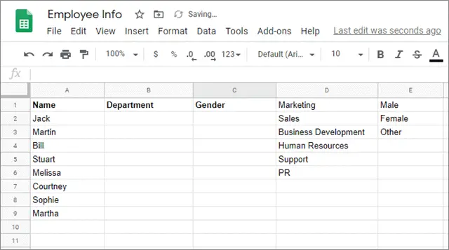
Adding a drop down menu in Google Sheets is a reasonably simple process. The main thing to know about is the context in which it is used. To begin with, open your Google spreadsheet. For instance, we have an Employee Info sheet prepared beforehand to explain the concept and use of drop-down lists.
Columns A, B, and C are reserved for the data entry of important information. Column D contains the entries that you will retrieve in the drop-down menu. It is from this list that you will recover the entries for column B. Similarly, the entries to be made in Column C have been created in Column E.
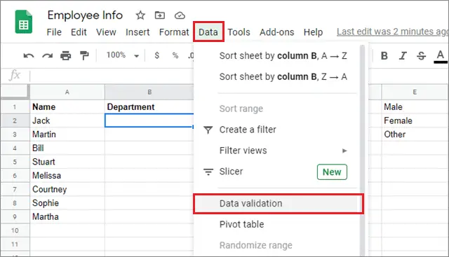
First and foremost, click on a cell or select a range of cells for which you want to add a Google Sheets drop down menu.
Then, click on the Data tab and select Data validation from the drop-down menu.
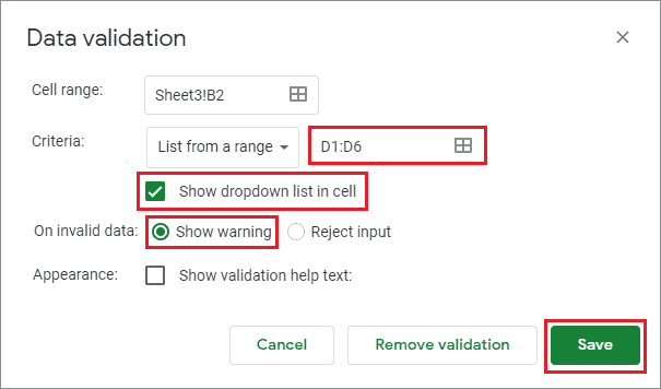
Now, make sure you enter the correct cell range in the first field. This will determine the cells in which you want to create.
Then, in the Criteria field, select the List from a range option. Next to that is another cell range. Here you have to insert the cell range you will retrieve for the drop down menu in Google sheets.
Now, we need to retrieve the entries in Column D for entering them in Column B. The cell range will be D1:D6.
After selecting the range of cells from, check the ‘Show dropdown list in cell,’ and choose Show warning in the ‘On invalid data’ field. After you have made all the changes, click on the Save button.
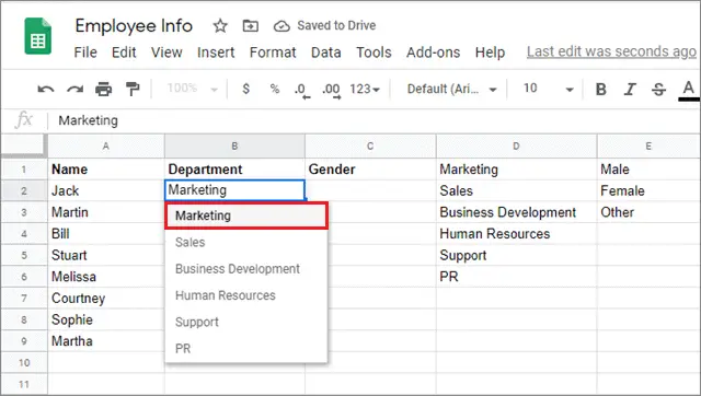
You will see that the Google sheets drop down menu has been created. Just click on the downward arrow and select your choice to enter data in the box.
You can follow the same method and also learn how to edit drop down list in Excel.
Types of Criteria
Data validation can be done based on different criteria. Let’s have a look at them and what they are used for in a Google Sheets drop down menu.
- List from a range: This option is used to retrieve values from a cell or a range of cells from the same or a different sheet in a workbook.
- List of items: It is for use when you want to validate data manually. The options to be used for drop down menu in Google Sheets must be separated by commas while entering then.
- Number: When you want to validate if a specific numerical entry falls into a specified numerical range, you can go with these criteria.
- Text: The option is used to validate whether a particular data entry contains or does not contain a specific string or text. It can also validate emails and URLs. The Text option does not have a typical Google Sheets drop down menu.
- Date: Similar to the Text criteria, this option also doesn’t create a dropdown menu. It validates if a data entry in the selected cell falls into a specific data range.
- Custom formula: This option allows users to verify a user-specified formula.
Whenever you choose criteria that creates a Google Sheets drop down menu, you will see the ‘Show dropdown list in cell’ option with a checkbox in the data validation dialog box. You can uncheck this box if you want the users to enter the data manually without having to refer to a drop-down list.
The ‘On invalid data’ field helps users know if anyone enters unknown data in a validated cell. The ‘Show warning’ option will mark an entry invalid if it doesn’t match the drop-down menu options. You can also use the reject input option to forbid the user from entering different data than what is expected.
Next, the Appearance checkbox below determines whether any text will appear to give the user an idea about the expected values in a cell range.
2. How To Enter Drop Down Menu Manually
At times, we need to validate data manually. If that’s the case, you can easily specify how you want to judge the data. In this method, users don’t need to create values in a different cell range and then retrieve them in another range of cells, as we did in the first method.
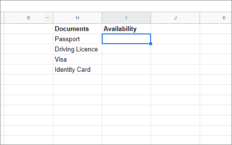
To begin with, open the Data Validation dialog box by following the steps in the first method. Here, we have a sheet where you need to manually verify if a person has a list of documents.
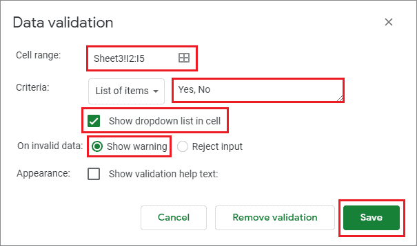
While creating a Google Sheets drop down list, change the criteria, and select ‘List of items.’ In the cell range column, select the range of cells in which you want to add the drop-down menu. Here, we have selected the range I2:I5.
Now, enter the values in the Criteria box. Here, we have decided to go with Yes and No as our values. As specified before, values need to be separated by commas, as shown in the figure below.
Check the Show drop-down menu in the cell checkbox, and select Show warning in the On invalid data field. The checkbox in the Appearance field will remain unchecked. Click on Save after you have entered all the details.
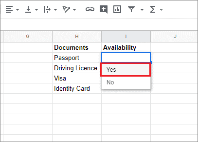
Now, you will see the downward arrow, indicating that the data validation has been applied. Click on that arrow and select the option accordingly.
That’s all about how to create drop down list in Google Sheets for verifying data manually. It can be used only at times when you have to judge data or validate facts.
3. How To Copy A Drop Down List
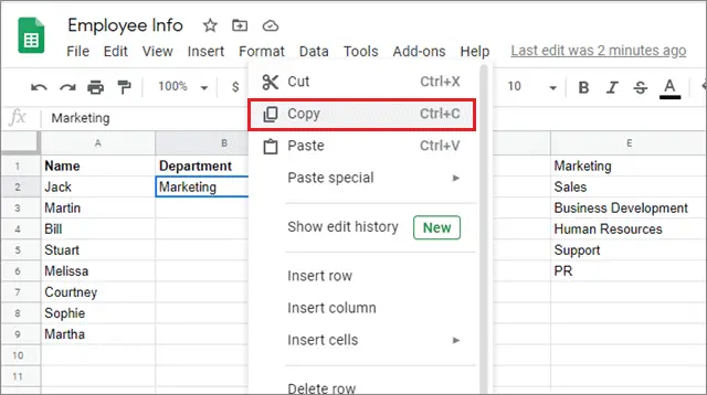
If you are retrieving data from a cell range to create Google Sheets drop down, you can copy that list with the usual Ctrl+C and Ctrl+V controls. However, if you want to copy a cell in which data validation has been applied, you need to tweak the copy-paste process.
First, select the cell, right-click on it and select the Copy option.
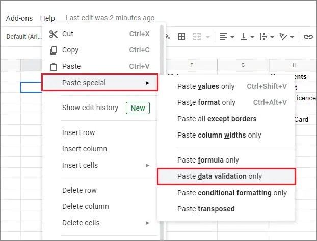
Then, select a cell in which you want to paste it. Right-click on that cell, select Paste special and click on Data validation only.
By doing this, you can paste the data validated cell anywhere in the sheet or different sheets in a workbook.
4. How To Force Users To Select Only Items From Your Drop Down Menu
You can use this method to restrict fellow users from adding values other than the ones specified by you in a cell or range of cells. To begin with, open the Data Validation dialog box from the Data tab.
Then, select the Reject input option in the On invalid data field.
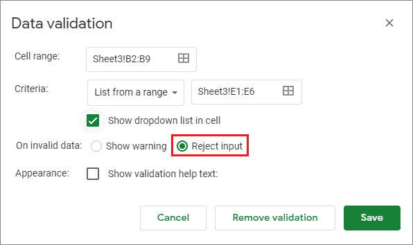
Now, other users won’t be able to add anything except the data specified in the drop-down list. Using this option cancels out the tiniest possibility of making an error while entering values in a datasheet.
5. How To Use Color Coding For Data Validation
Before we move on with this method, you must know that color-coding cells aren’t mandatory. However, it can be used for a better visual understanding of the data.
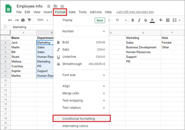
To begin with, select the range of cells you want to color and go to the Format tab. Select the Conditional formatting option from the drop-down menu.
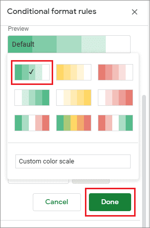
Now, in the right side of the pane, select the cell range. You can change the color of the cells by selecting one under the formatting style.
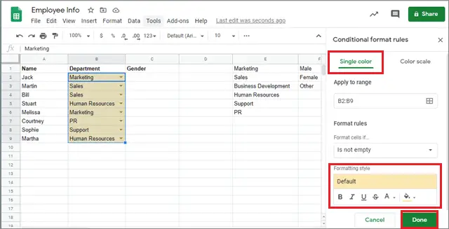
Next, select the Color scale tab and choose the color range as per your choice.
Having color-coded cells means your data is visually pleasing to work on, not to mention the impressive organization that helps other users in understanding it better.
6. How To Remove Data Validation
Now that we have learned the basics and details of how to add drop down list in Google Sheets, let’s see how to remove it.
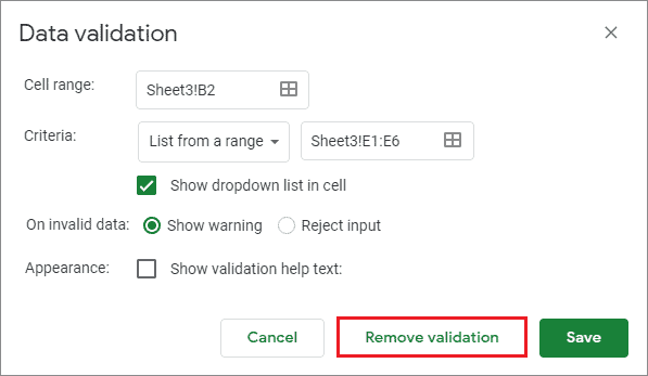
All you have to do is select the cell in which the validation is applied and open the Data Validation dialog box. Then, click on the Remove data validation option.
The downward arrow that indicates the presence of a drop down list vanishing, meaning you have successfully deleted the validation.
7. How To Create A Drop Down List On Android Smartphones
Creating a drop down list on an Android is similar to doing so on a desktop. You will need to download the Google Sheets app for this purpose.
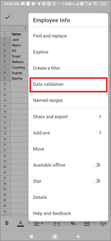
If you already have it on your phone, click on it and open a spreadsheet. To add a Google Sheets drop down menu, first select a range of cells, and then click on the three vertical dots in the top right corner.
Then, click on Data validation.
Next, select the Criteria you want to add. If you choose a List of items, you need to click on the +Add option and enter the items. Click on Done to save an item.
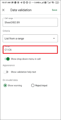
If you select List from a range, you need to enter the cells you want to include. You can set the ‘On invalid data’ field as per your requirement. Here, we have chosen Show warning. After making all the necessary settings and adding the list of items, click on the Save button.
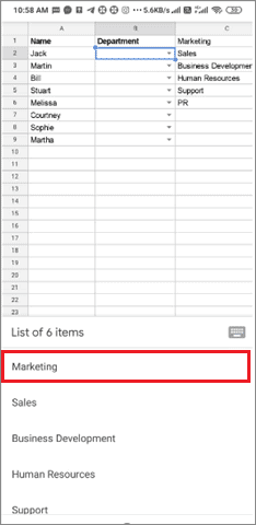
You will see that the downward arrow has appeared in the selected cells. By clicking on that arrow, you can choose your data entry.
The Google Sheets app is a handy app you can use to learn how to create Google Sheets drop down list. In case you don’t possess a laptop, you can always use this app to create a drop down menu in a spreadsheet.
Conclusion
Whenever we are filling in or creating complex datasheets, it is necessary to maintain a thorough check of the values being entered in it. If any value, be it text or numerical, is entered incorrectly, it can cause discrepancies in the results at the end.
The Google Sheets drop down feature is used to prevent these inaccurate manual entries and ensure that the correct data is entered regularly. Users can validate the data by creating drop-down lists for various purposes, as shown in the steps above, and maintain accuracy in the data.
You can also follow the same basic method to add and edit dropdown list in Excel. The choice of using drop-down menus depends on the needs and requirements of both users and data.
(Updated on 7th January 2021)


