The best part about Google Sheets compared to Microsoft Excel is that the former allows you to collaborate and work together on spreadsheets simultaneously with your contacts. However, you could risk missing out on important stuff in your spreadsheets while collaborating with your contacts. You can avoid that issue if you know how to lock cells in Google Sheets.
If some of the columns are unimportant, you can choose to hide or freeze these columns for better convenience. However, if you have a specific set of cells you want to protect, locking cells is the best option instead of hiding or freezing an entire row or column in a spreadsheet.
How To Lock Cells In Google Sheets To Ensure Data Protection
Locking cells is a simple process; it protects data when multiple users edit a Google Sheets spreadsheet. On that note, let’s look at how to lock cells and protect data in them.
Steps To Check Word Count On Google Docs
1. Open Google Sheets.
2. Right-click on the specific cell and select Protect range.
3. Click on Add a sheet or range.
4. Enter a description and select the range.
5. Set the required permissions.
Now you know the basics of how to lock cells in Google Sheets. Let’s check and study the steps in detail with images.
How To Lock Cells In Google Sheets
Let’s get to the main process of lock cells in Google Sheets. We will use this sample sheet given below to understand the process of locking cells.
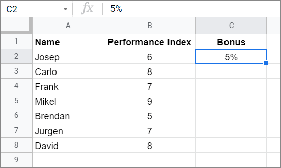
The main aim here is to lock cell reference C2, which contains the bonus figure.
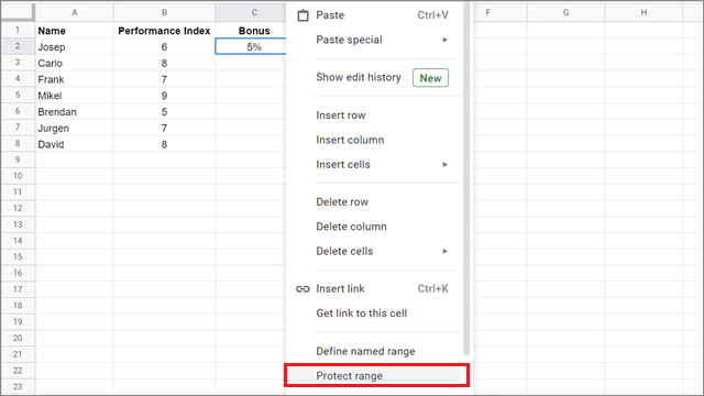
Right-click On The Cell And Select Protect Range
To begin with, open the Google sheets. You know how to lock cells in Google Sheets, right-click on the selected cell and click on Protect range from the drop-down menu.
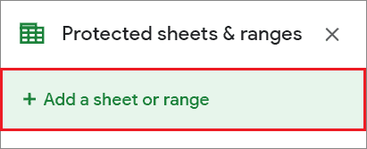
Add A Sheet Or Range
Next, click on ‘Add a sheet or range’ in the right sidebar.
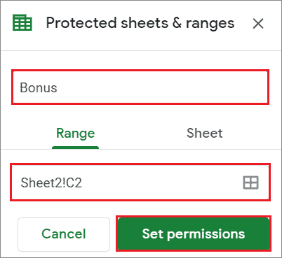
Enter A Description And Select The Range
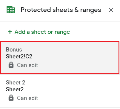
Enter the description of the cell in the first blank field. Here, we have entered ‘Bonus’ in the description field.
Then, select the cell or range that you want to lock. In our case, the cell is C2. Click on Permissions after you have entered the details.
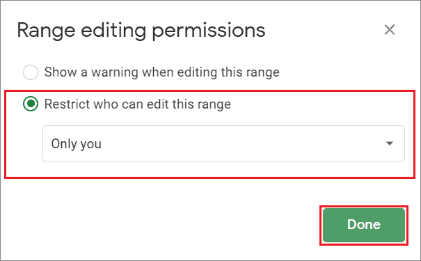
Set The Required Permissions
In the ‘Range editing permissions’ dialog box, select ‘Only you’ in the ‘Restrict who can edit this range’ section.
Click on Done after you have made the setting mentioned above.
We have seen how to lock an individual cell in a Google spreadsheet. However, you can also lock multiple rows and columns by selecting a cell range in the third step. As a step further, you can use a conditional formatting rule to mark the locked cells so that other collaborators know they are not allowed to edit those cells.
Give Editing Permissions To Specific People
Once you know how to lock cells in Google Sheets, you can give editing permission to selected users in a Google sheet document.
To begin with, follow the first three steps in the previous example. Then, follow the instructions given below.
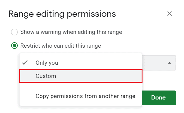
Select The Custom Option
Once you open the Range editing permissions dialog box, select the Custom option.
Add The Editor
In the dialog box that appears, add the name or the email address of the person you wish to permit to edit the cell.
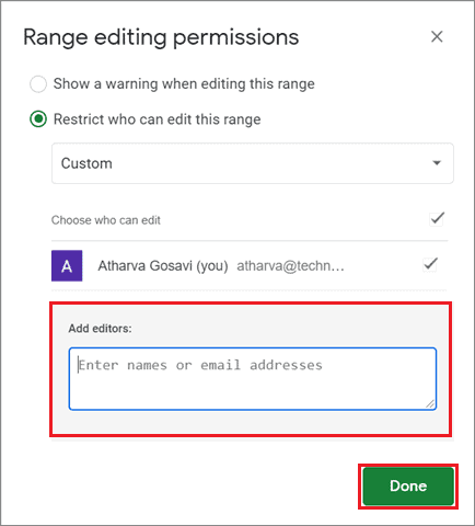
Click on Done after adding the details.
Protect And Lock Entire Sheet in Google Spreadsheet
Just like how to lock cells in Google Sheets, you can also do the same for an entire Google Sheets worksheet.
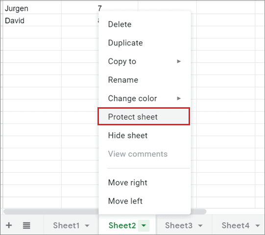
Click On The Downward Arrow on the Sheet tab
To begin with, click on the downward arrow on the Sheet tab and click on Protect Sheet from the menu.
Enter The Sheet Number And Description
Click on the Sheet tab in the right sidebar and select the Sheet which you want to protect. You can also enter the description of the selected sheet in the empty field above it.
Click on Set permissions after entering the required details.
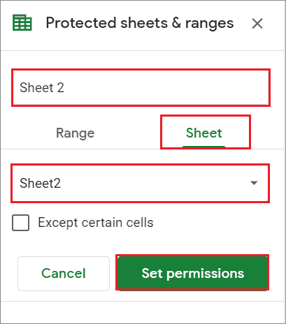
If you want to lock the entire sheet but leave some cells unlocked, you can check the ‘Except certain cells’ tick box.
Set The Required Permissions To Ensure Sheet Protection
Now, set permission as required and click on Done.
You can also permit certain collaborators to edit the sheet by using the same method we saw for cells in the second method.
How To Unlock A Locked Cell
To unlock a locked cell or a protected worksheet, you must follow similar steps as we saw previously, except for one simple tweak.
Select The Range
When you open the ‘Protected sheets & ranges’ sidebar, click on the range option.
Click On The Delete Icon
Now, click on the Delete icon to unlock cells.
How To Show A Warning But Allow Editing Of Cells
If you don’t wish to lock cells but let other collaborators know that they are not allowed to lock this cell, you can show them soft warnings before they edit it.
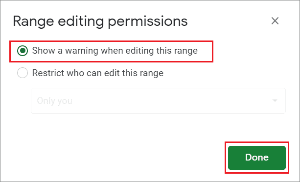
To enable the warning option, open the ‘Range editing permissions’ window and enable the option called ‘Show a warning when editing this range.’
Click on Done once you enable the option.
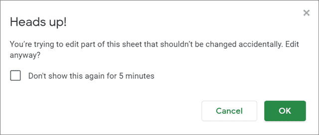
This is how the warning option looks like if a collaborator tries to edit a protected cell.
These are the ways of knowing how to lock cells in Google Sheets. As an alternative, you can also try protecting Google Sheets using a password for ensuring data protection of a cell value.
Conclusion
Locking cells is a simple process that you can execute in the blink of an eye. The main reason why we do it is to protect sensitive data in spreadsheets that shouldn’t be changed at any cost. If you know how to lock cells in Google Sheets, you can save essential data when multiple collaborators work on a shared spreadsheet.
Freezing or hiding is an excellent alternative to locking cells, albeit it is only valid when you want to freeze or hide an entire row or column. When it comes to locked cells, you can also allow specific people to edit them. You can also display a warning to collaborators who don’t have permission to edit locked cells so that they may refrain from editing them.


