VLOOKUP function is one of the most frequently used formulas for analyzing data in Google Sheets or Microsoft Excel spreadsheets. It is arguably a complex function to master, nonetheless an important one that you can’t skip. If you wish to become a data or business analyst, it is an added advantage to know how to use VLOOKUP in Google Sheets.
The term ‘VLOOKUP’ stands for Vertical Lookup. The VLOOKUP function lets you search the leftmost column of a range to return a value from any other column in that same range. This saves the monotonous work of scrolling left every time to retrieve values when you are working on complex and large datasheets.
VLOOKUP In Google Sheets: Analyze Data With Ease
The Google Sheets VLOOKUP function allows you to search and link two different datasets with a single search value. It is made up of four segments. Once you calculate the result in a cell using the VLOOKUP function, you can use the Google Sheets fill-down method to calculate the results for other cells. Let’s look at what these segments are and how to use the lookup function.
How To Use VLOOKUP In Google Sheets
1. Open Google Sheets.
2. Enter the VLOOKUP Google Sheets formula in the cell.
3. Press Enter to view the result.
You can use the VLOOKUP function by following these simple steps. Now, let’s take a look at the function syntax.
Syntax of the VLOOKUP Function
The syntax of VLOOKUP in Google Sheets is given below. This function searches for a value vertically, i.e., up and down a selected column. The HLOOKUP function works similarly to the VLOOKUP, albeit horizontally.
=VLOOKUP(search_key, range, index, [is_sorted])search_key: This is the term in the original table you wish to find in the lookup table.
range: The range of the lookup table in which you will search for the term from the original table. VLOOKUP Google Sheets or Excel formula constantly searches down the first column of this table for the search key.
index: index value is the column number in which you want to search for the search_key. For example, If you wish to search for the term in the first column, the index value would be 1. If you want to search for the term in the second column, the index value would be 2.
If the index value is greater than the number of columns in the lookup table, you will get a #REF! Error.
is_sorted: This argument is used to determine if you want to find the exact search term or the nearest match to it. A TRUE or FALSE value always indicates it. 1 shows a TRUE value, and 0 indicates a FALSE value. If the user skips this argument, the default value is considered to be TRUE.
If the is_sorted value is FALSE
- It commands the function to find an exact match of the search term
- It is not case-sensitive
- If multiple values match the search term, the first value is always returned as a result.
- If no match is found, you will get a #N/A Error message.
If the is_sorted value is TRUE
- The function will find the nearest match that is equal to or less than the search term
- This value is used rarely
7 Ways To Use The VLOOKUP Function
There are seven different scenarios in which users can opt for the VLOOKUP function. Let’s get to know each system in detail.
1. How To Use The VLOOKUP Function In Single Sheet
Now that we know the basics of the VLOOKUP function, let’s look at how we can use it for different purposes.
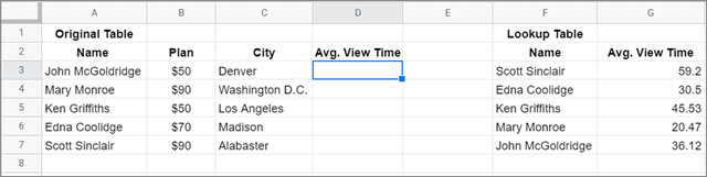
Let’s use a sample data table to understand the working of VLOOKUP in Google Sheets. This is a list of customers who have opted in for a video streaming service. The main aim here is to retrieve the Avg. View time from the lookup table into the original table.
Enter The Formula
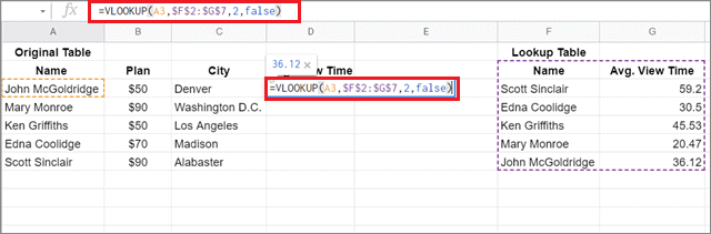
To begin with, select the cell in the column where you want to retrieve the data. Then, enter the formula. In our case, the formula is as given below.
=VLOOKUP(A3,$F$2:$G$7,2,false)The ‘$’ symbol is inserted to make sure both the row number and the column heading are fixed and don’t change. It is useful when you want to copy and paste the formula to a different sheet or cell. The $ symbol ensures cell references aren’t changed when you copy and paste them.
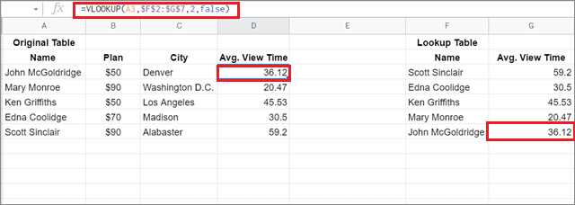
View The Result
Once you press the Enter key, you can check the result. The values from the Lookup table will be retrieved in the Original table.
You can also use the VLOOKUP Google Sheets function with an array formula to calculate results for a specified range of cells.
2. How To Use VLOOKUP Function For Multiple Sheets
The Google Sheets VLOOKUP function can be used to retrieve data from multiple sheets or sources. The formula is similar to what we saw in the previous method, albeit with a minor tweak.
For this case, let’s refer to this sample sheet.
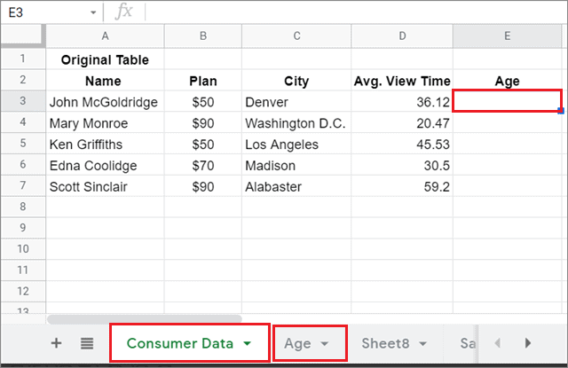
We have already retrieved the Avg. View time from the Lookup table. Now, the aim is to retrieve the age of customers from a different sheet.
Enter The Formula
To begin with, select the cell and add the formula. In our case, this is how the formula will look like –
=VLOOKUP(E3,Age!A1:B6,2,false)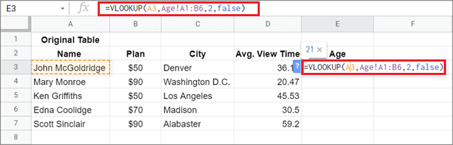
View The Result
Press Enter key to view the result.
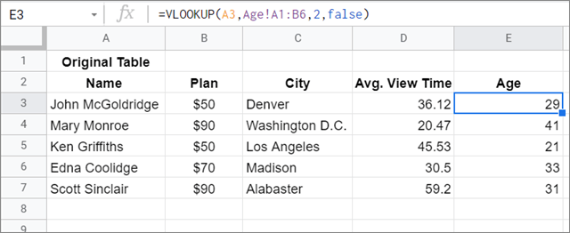
Here, the second string, ‘Age!A1:B6’, contains the sheet’s name and the data range from another sheet. ‘2’ is the index value of the column in that data range.
3. How To Use VLOOKUP With WildCards
In the previous examples, we have an exact value to search from the lookup table. If you don’t have an actual value, use a wildcard character to find partial matches in a spreadsheet file.
To understand it better, let’s consider this sample sheet.
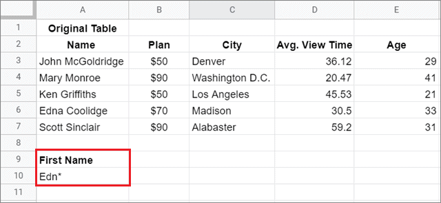
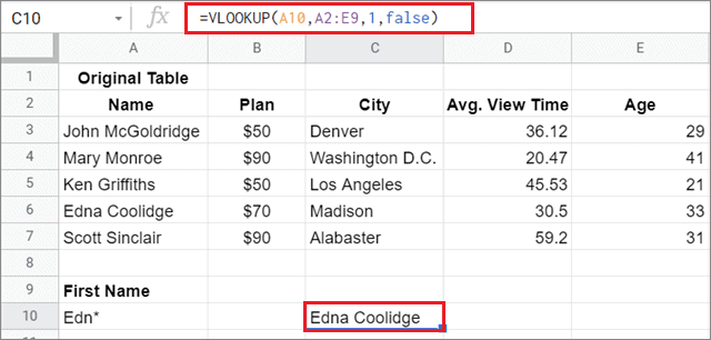
Now, suppose you are given just a name or a sequence of letters in a name, you can use wildcard characters like a question mark(?) or asterisk(*) to find the matching value. The question mark is used to match a single character, while the asterisk matches a sequence of characters.
In this case, we will retrieve a value with the words ‘Edn’ in the result column.
Enter The Function
To begin with, formulate and enter the VLOOKUP in Google Sheets.
=VLOOKUP(A10,A2:E7,1,false)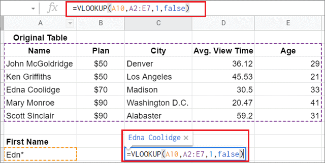
Check The Result
Obtain the results by hitting the Enter key. You can see that the VLOOKUP Google Sheets function returns the value in the selected table that contains the search term.
4. How To Use VLOOKUP To Find Closest Match
Sometimes, we might not have an exact matching term to find from a table. However, you can still use the VLOOKUP function to find the nearest matching terms that fit within specific criteria or satisfy a condition.
Let’s consider this sample sheet.
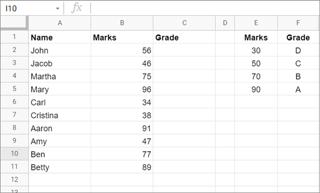
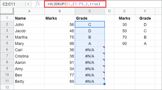
Here, we have to assign grades to students based on their marks using the grade table.
If you want to find the closest match, you need to use the TRUE argument in the function. Also, make sure the search column is sorted in ascending order.
In our case, the Marks and Grade table in E1:F6 is our lookup table. Column E is our search column, and it has been arranged in ascending order.
Enter The Function
First and foremost, select the column and enter the VLOOKUP in Google Sheets, as shown in the image below.
=VLOOKUP(B2,$E$1:$F$5,2,true)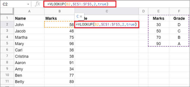
View The Result
Now, press the Enter key to view the result. You can drag the cell accordingly to fill up the grades for the rest of the students.
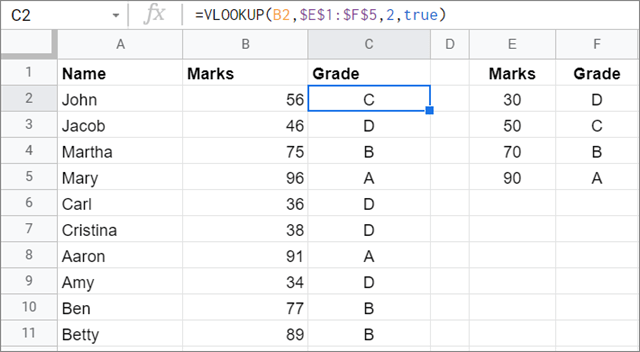
Make sure you remember to insert the ‘$’ symbols here. They restrict the range from changing when you drag the result to obtain values in all the columns.
If the ‘$’ symbol isn’t present in this case, the grades will be assigned only once, and the ‘#N/A’ result will be returned in the rest of the columns, as shown in the image below.
Notice that after removing the $ symbol from the entire column, the grades are assigned only once, and the error result is returned for the rest of the cells.
Moving forward, you can use the conditional formatting in Google Sheets to mark students who have received a particular grade. The conditional formatting function is generally used when it comes to highlighting multiple criteria in a spreadsheet.
5. How To Do A Two-Way Lookup
When you search a table with multiple columns and multiple rows, you can use the nested MATCH function with VLOOKUP.
To understand this point better, let’s take a look at this sample sheet given below.
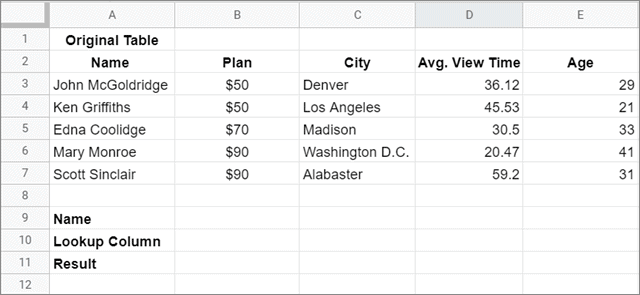
Here, we have to decide the lookup column first and then enter the name. Once you enter both terms, the lookup table will automatically pull the result cell next to Result.
So, as an example, let’s consider Avg. View Time as the Lookup Column. When you enter the name of a customer, you will get their Avg. View Time as a result.
Enter The Formula
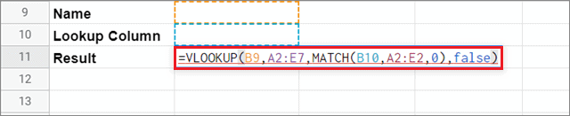
First and foremost, select the cell in which you want to obtain the result and enter the formula given below.
=VLOOKUP(B9,A2:E7,MATCH(B10,A2:E2,0),false)Now, let’s look at the breakdown of the formula.
B9: This is the name you have entered in the search field. Once you enter the name, the VLOOKUP in Google Sheets will look for this term in the leftmost column of the specified range.
A2:E7: The table from cell A2 to E7 is the specified range of the table from which we will retrieve the result.
MATCH(B10,A2:E2,0): The MATCH function will use the Lookup Column to find the parameter in the header range of the main table. Here, B10 specifies the Lookup Column and A2:E2 specifies the entire row of headers. The ‘0’ indicates that the range is not sorted.
false: It indicates that the range for the entire VLOOKUP function is not sorted.
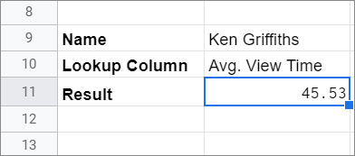
Press Enter key after inserting the function. You will receive a ‘#N/A’ error in the selected cell range. That error will be resolved when you follow the next step.
Enter The Details And View The Result
Now, enter details in the remaining two fields. You will automatically get results in the Result field.
6. How To Use VLOOKUP To Compare Two Data Lists
Suppose you have two complex datasheets and you wish to find out if a particular term exists in both datasheets. You can use the Google Sheets VLOOKUP function with the IFERROR function in this case.
Let’s take a look at this sample sheet given below.
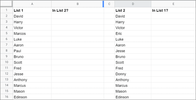
Here, we have two data lists in the Google spreadsheet, and we need to find out if a particular term from List 1 is present in List 2 and vice versa.
Enter The Function
To begin with, select the cell in which you wish to obtain the result. Here, we have selected cell B2. Now, enter the VLOOKUP in Google Sheets spreadsheet. This is how it will look like-
=IFERROR(VLOOKUP(A2,D:D,1,false),"Not in List 2")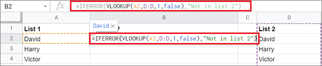
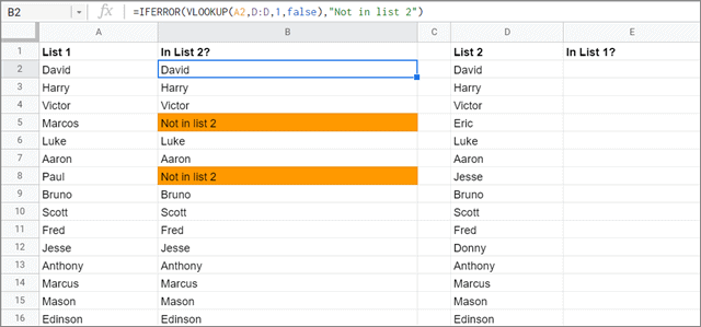
View The Result
Once you press Enter, all the values present in List 2 will be returned in the result column.
You can follow the same method to obtain the result in column E.
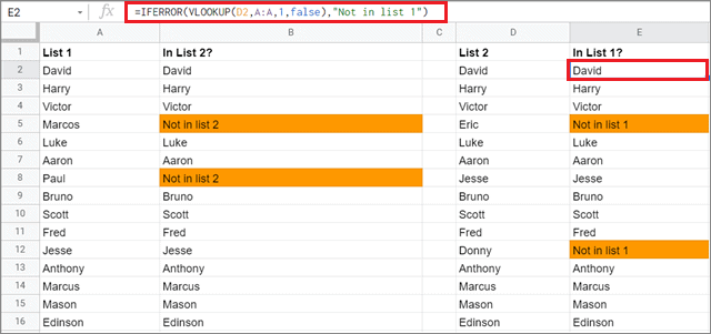
This is how you can use the VLOOKUP function in various circumstances.
7. How To Use The VLOOKUP Function Using An Add-On
If you don’t want to use the VLOOKUP function, you can install an add-on called Merge Sheets by Ablebits to retrieve data quickly. After installing the add-on, you can follow these steps to perform the VLOOKUP function.
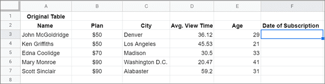
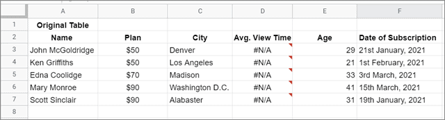
We will consider this sample sheet to understand the working of the add-on. Here, we will retrieve the Date of Subscription from a different spreadsheet.
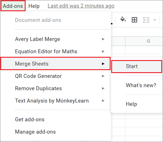
Step 1: Open Merge Sheets Add-On
To begin with, click on the Add-ons tab, select Merge Sheets, and click on Start.
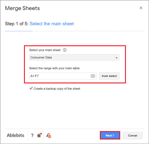
Step 2: Select The Main Sheet And Cell Range
To begin with, select the main sheet and choose the cell range of the table you want to work on.
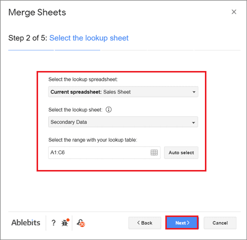
Step 3: Select The Lookup Table And Cell Range
Now, select the sheet from which you want to retrieve the data and the cell range.
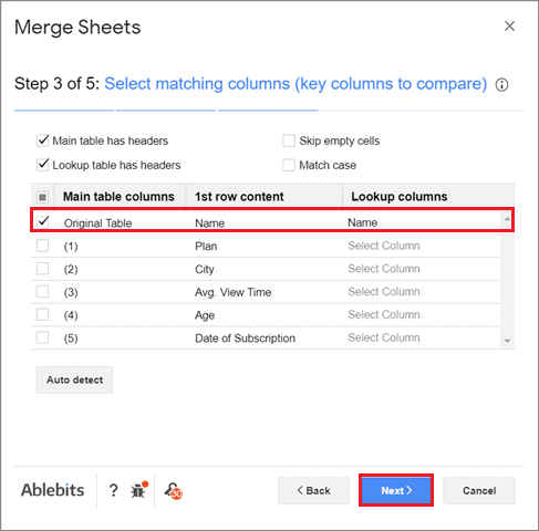
Step 4: Select Match Columns
Now, select the common columns in both sheets for reference. Here, we have selected the Name column.
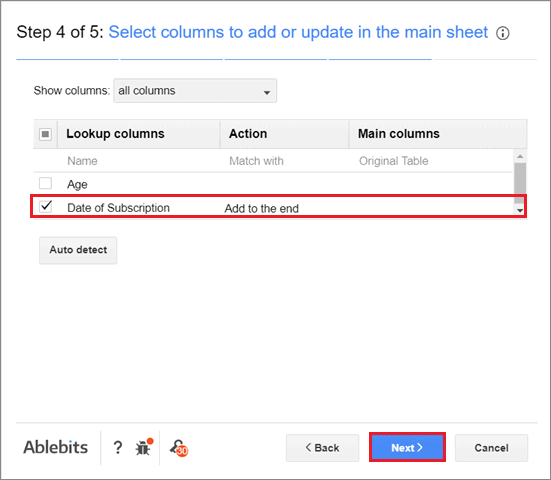
Step 5: Select Columns To Update In The Main Sheet
In the next step, select the column in the secondary sheet that you want to update in the main sheet. Here, we have selected the Date of Subscription column.
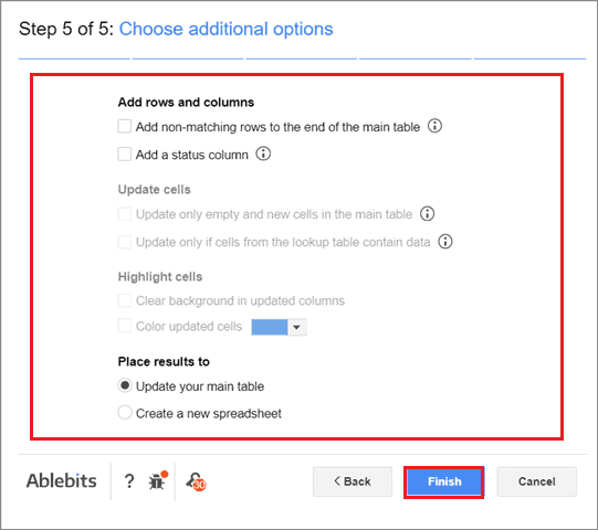
Step 6: Choose Additional Options
You can also add any non-matching rows by selecting the first checkbox below. Once you select it, click on the Finish button.
Step 7: View The Result
You can see the selected column has been filled successfully.
Limitations of Google Sheets VLOOKUP Function
The VLOOKUP in Google Sheets also has a fair share of limitations that users need to be wary about.
1. The VLOOKUP function only considers columns to the right of the lookup value. Suppose your lookup column is column B, you cannot use the VLOOKUP function to extract information from column A because it lies to the left of column B.
2. The function lacks dynamics; it fails to update the column index values if we insert a new column in the specific cell range.
Conclusion
We have seen how the VLOOKUP in Google Sheets can be used to analyze data in different ways to derive meaningful conclusions from it. There’s a widespread misconception that this function is tough to use and master. However, that can be easily tackled if you practice it every day.
The Google Sheets VLOOKUP function is predominantly used in complex datasheets where you need to retrieve values from cells far apart across a Google sheet. It also helps in linking two separate datasets using a common search value. Finding information across complex worksheets becomes a cakewalk if you know how to use this function properly.


