Microsoft Excel is a widely used software for creating, storing, and editing datasheets. On both personal and professional levels, users require sorted datasheets for clarity. They can also refer to specific entries in the sheets quickly. So, one must know how to alphabetize in Excel and sort the data.
There are various ways in which users want to sort their data, depending on the type of datasheets they are working on. In most cases, data can be sorted with just one click, while at times, you need to carry out some complex tasks to alphabetize it. The A-Z and Z-A sorting buttons are used the most while arranging data in a proper manner and format.
How To Alphabetize In Excel To Arrange Data
That being said, let’s dive in to learn a host of methods with which we can alphabetize our data for both personal as well as professional purposes. Mind you, some of the processes are lengthy, but once you learn them, you can carry them out in the blink of an eye!
1. How to Alphabetize in Excel Using a Column
Sorting a column in Microsoft Excel is one of the easiest tasks to carry out. If you want to sort the data in alphabetical order as per the columns, the fastest way to do it is to use the sorting tool present in the ribbon.
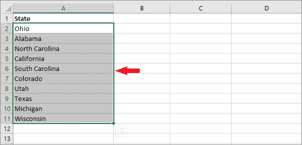
To start with, select the column with the entries that you want to alphabetize in any order.
Then, go to the Data tab on the ribbon and select the Sorting tool. The Sorting tool can also be found on the home tab.
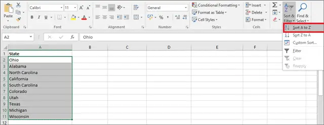
You can arrange the entries in ascending order by choosing A-Z or in descending order by selecting Z-A.
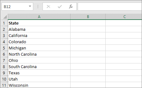
Once you make your choice and select the option, you will instantly see the results as the column arranges itself. The same method is also applicable if you want to alphabetize on Google Sheets/Docs.
2. Sort A Column Alphabetically by Using A Filter
You can use the filter method if you want to alphabetize columns with speed. By applying filters to columns, the sort options for all the columns can be accessed with just one click.
Go to the Data tab and click Sort and Filter. Then, select the Filter option.
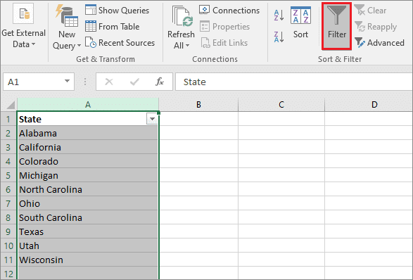
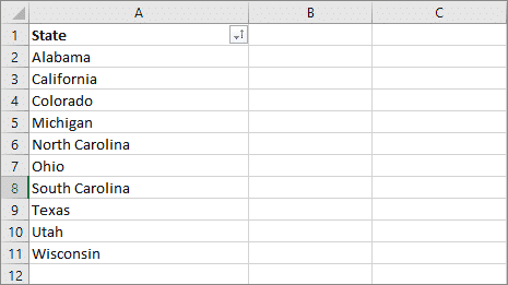
Small drop-down arrows will appear on each of the columns. Click on the arrow of any column you want to sort and select A – Z.
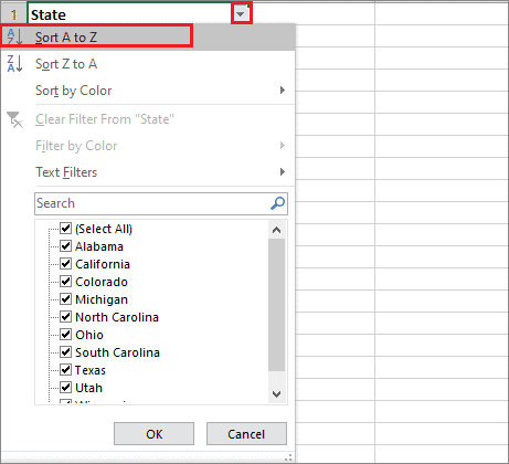
This will arrange the column you want in alphabetical order.
If you wish to remove the filter, click on the Filter button again, and the function will be disabled. The best use of filtering is when you want a large group of people in alphabetical order.
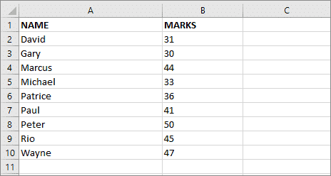
3. How to Sort in Excel and Keep Rows Together
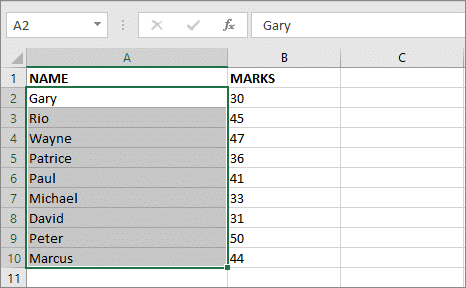
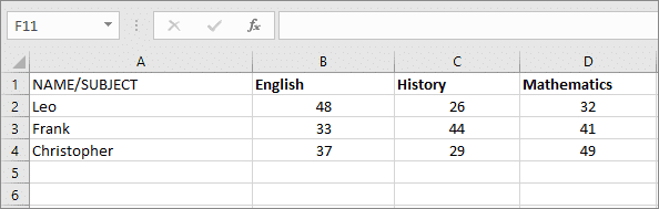
Sometimes, we work on datasheets where we need to keep rows intact after arranging the columns. For example, If we want to sort a list of students alphabetically, we also need to make sure that the marks entered in the rows next to them should also move accordingly once the sorting is done.
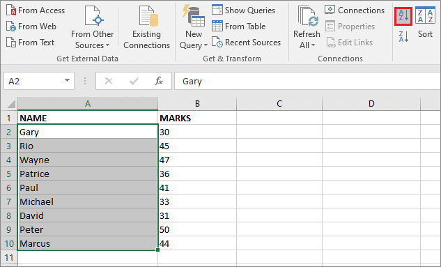
To start with, select the first column with the help of the header row according to which you want other columns to be sorted.
In such cases, you can click Sort and select either A-Z or Z-A to arrange the data in one column you want, and Excel will automatically rearrange the other columns accordingly.
Once you click the sorting option, a Sort Warning dialog box will open up. Select Expand the selection and press Sort.

As you can see, Excel keeps the rows together while sorting columns, so you don’t have to worry about any mismatched data.
When arranging columns, users need not worry about how to alphabetize in Excel and keep the rows intact. The software offers an in-built feature for the same.
4. How to Sort Data in Excel Using Multiple Columns
Alphabetizing multiple columns using Excel is an easy task, albeit it does have more number of steps to carry out as compared to all the other methods. The Sort command will do the needful for you in this case.
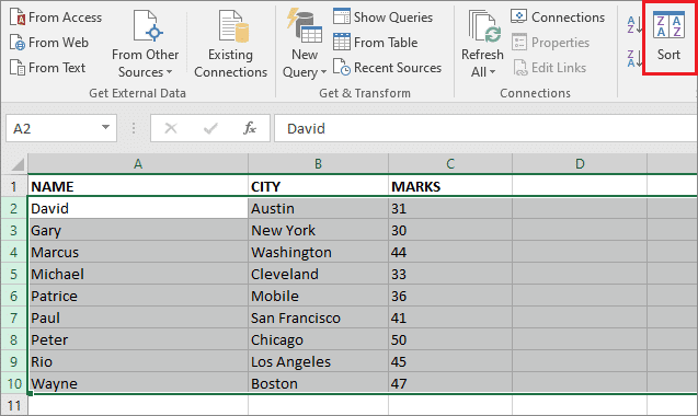
Assuming that you have a table prepared with multiple columns, select it entirely. Then, go to the Data tab and in the Sort and Filter group, click on Sort.
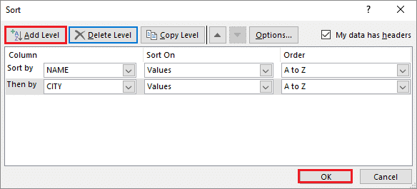
The Sort dialog box will open up and show the first parameter in which the table will be sorted. In the dropdown menu, select the first column in the header row according to which you want the table to be alphabetized.
In the next two boxes, select Cell values for Sort on and A-Z for Order. Click on the Add option and follow the same steps to enter the parameter in which you want the table to be sorted. Then, click on Ok.
Excel will sort the data as specified. Likewise, you can sort the data by adding as many parameters as you wish.
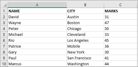
That is how to alphabetize in Excel when it comes to re-arranging data based on multiple columns. The process might appear a tad bit long, but it’s easy to execute once you do it practically.
5. Alphabetize Rows
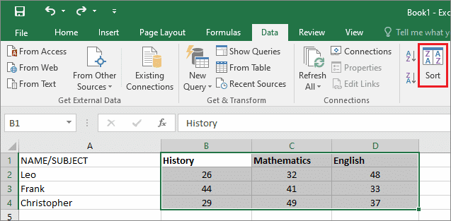
If your data is arranged horizontally, you need to arrange it by taking rows into consideration. This can be done by using the same Sort and Filter feature in the Excel ribbon.
To start with, select all the rows that you want to alphabetize; make sure you leave out the column in which you have labeled all rows.
Now, navigate to the Sort and Filter option and click Sort.
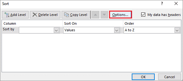
In the dialog box that opens, click on Options.
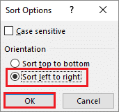
Another small dialog box will open up. Select the ‘Sort left to right’ option and click Ok to get back to the Sort dialog box.
Now, select the Row you want to alphabetize in the Sort by drop-down list. In the other two boxes, select Sell values and A-Z.
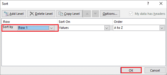
As the result shows, the first row is alphabetized and the remaining rows are rearranged accordingly.
Also, make sure you don’t keep any of the cells blank while sorting as it can cause problems and errors in the final result.
6. How To Alphabetize Entries With the Last Name
Sometimes, we often have to alphabetize datasheets with last names. In such cases, even though the name appears first in a cell, the last name has to be given priority. You can carry out this task using Excel formulas.
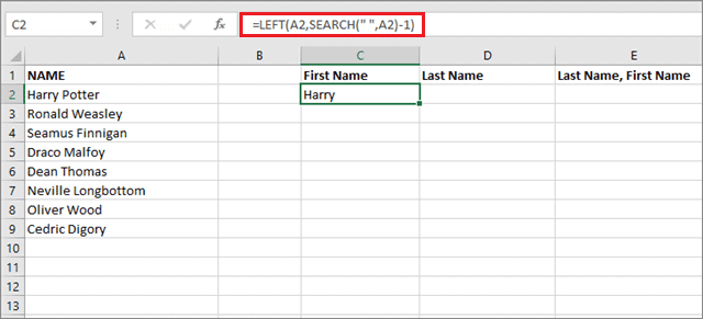
To start with, you will have to extract the first and the last names of each person you want to alphabetize in Excel into two different cells. In this case, the first name is extracted in the C2 cell and the last name in the D2 cell.
In C2, extract the first name using the following formula:
=LEFT(A2,SEARCH(” “,A2)-1)
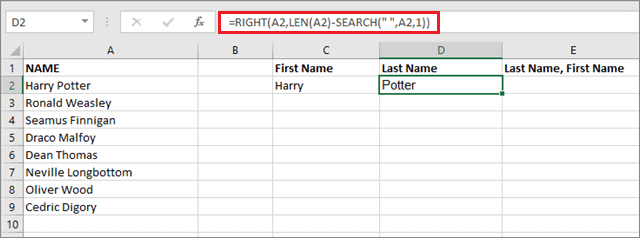
In D2, pull the last name:
=RIGHT(A2,LEN(A2)-SEARCH(” “,A2,1))
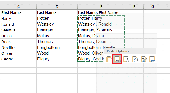
Then, the E2 cell, concatenate the parts in the reverse order like this:
=D2&”, “&C2
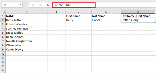
The basic idea is to reverse the names, sort them, and then reverse them back to their original form.
Now, the E column contains all the inverted names with the last names appearing first and the first names appearing after it. Now, select all the names in the E column, right-click on the selected portion, and select Values under Paste options.
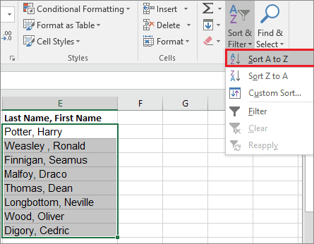
Then, select any cell from the resulting column and select A-Z or Z-A as per your requirements. The entire column will be alphabetized by the last name.
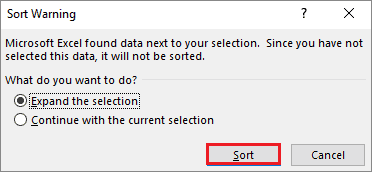
A Sort Warning dialog box will appear once you select the option. Choose Expand Selection and click on the Sort option.
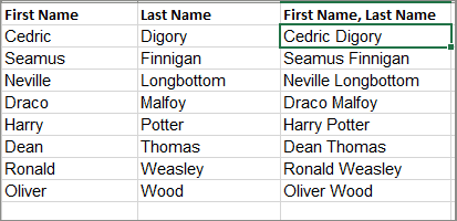
This is how the table will look after you have performed all the steps.
Now, if you wish to reverse it back, select a new column and then enter the following formulas.
Extract the first name:
=RIGHT(E2, LEN(E2) – SEARCH(” “, E2))
Extract the last name:
=LEFT(E2, SEARCH(” “, E2) – 2)
And bring the two parts together:
=G2&” “&H2
Then, select all the results in the I column and perform the formulas to values conversion once more. Further, follow the same procedure as we did above, and you will get the results.
Final Thoughts on How to Alphabetize in Excel
Microsoft Excel is one of the most vital software when it comes to creating, storing, and editing massive chunks of datasheets. Also, how to alphabetize in Excel is a common query asked by users who are tasked with arranging and formatting the data in order.
There are many types of sorting datasheets and several methods to execute them. These methods might come handy at particular instants when a user has to edit different types of datasheets while adhering to certain parameters. Users can sort data in Excel based on columns as well as rows using simple sorting options and some advanced formulas. The decision to do so entirely depends upon the needs and requirements of the user.


