How to Filter In Google Sheets And Organize Data

If you are not working with database software, the best way to work with data is by using a Microsoft Excel or Google Sheets spreadsheet. However, when it comes to the large data size, it becomes crucial for users to organize that data to gain valuable insights. Hence, you need to know how to filter in Google Sheets to manage your data.

Before you apply filter conditions, it is equally essential to sort the data you are working on. Data can be sorted alphabetically or numerically for the selected range of cells. The sorting of data in Sheets is straightforward to understand and execute and should always be used before data filtering. You can also know how to create drop-down lists using data validation to sort and filter data.

How to Sort And Filter In Google Sheets To Organize Data

Filtering comes into play when you have to see only a subset of rows in a large amount of data on a spreadsheet. It helps narrow down the range of values and data to view only the important chunk. You can also look at how to use the FILTER function in Google Sheets if you wish to know more about the advanced filter formula and filtering methods.

Note: By following these simple steps mentioned above, you can apply the Google Sheets filter to a large dataset and retrieve specific entries that you want to check. Let’s look at the steps for how to filter in Google Sheets with detailed images.

How To Use Google Sheets Filter

Users can use the Google sheets filter to segregate their data in a spreadsheet using the simple steps mentioned below.

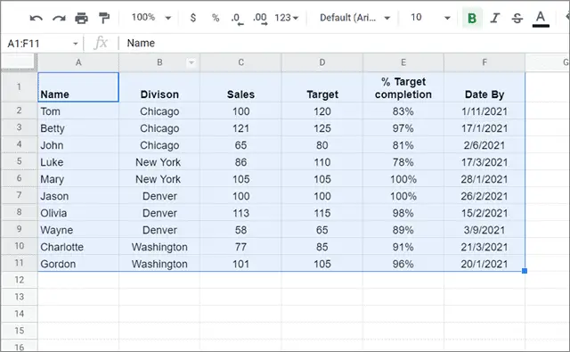
First, open the Google Sheets spreadsheet and select the data that you want to filter.

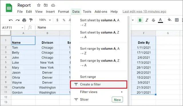
Navigate to the menu bar and click on the Data tab on the toolbar. Next, click on the ‘Create a filter’ button from the drop-down menu.

As an alternative shortcut, you can select the cell range and click on the filter icon in the toolbar to add a basic filter.

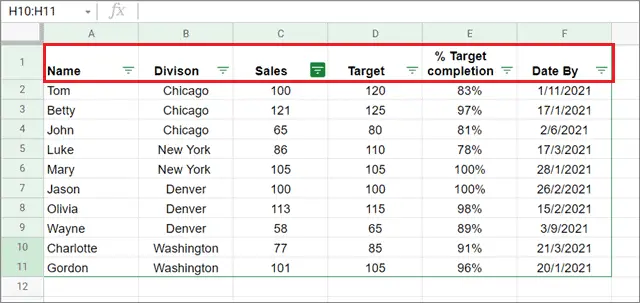
Now, you will see the filter sign (three horizontal bars) in all the column headers.

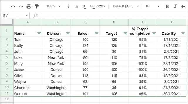
Click on the filter function in Google Sheets. You can use it in different ways.

Filter By Condition

If you choose the ‘Filter by condition’ option, you must specify the condition to obtain the filtered data.

There are multiple conditions available for filtering. You can choose the custom filter option at the bottom to create a custom formula that isn’t already available. These condition filters are also known as advanced filters.

Let’s consider an example. In the Google sheet below, we have to narrow down the data and view only executives who have made more than or equal to 80 sales. So, we need to filter data based on numeric values in column C.

You can use a filter formula using the operators given in this section. So, select the Greater than or equal to condition and enter 80 in the filter value box.

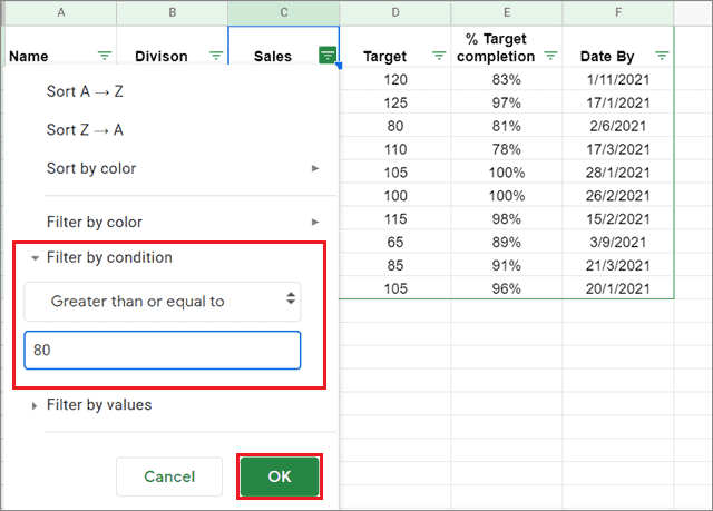
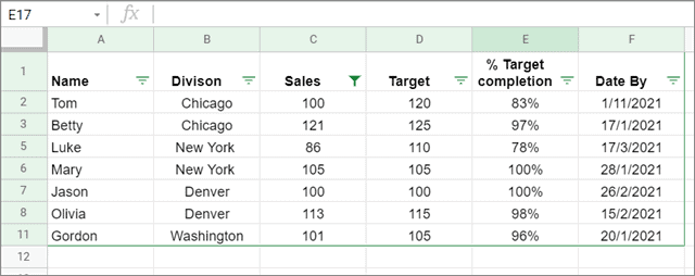
Once you click on OK, you can check the results.

Filter By Value

If you select the ‘Filter by value’ option, you must specify the value to filter data in a Google sheet.

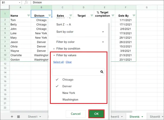
For example, let’s say you want to view sales figures made only from Chicago and Denver.

So, click on the three horizontal lines to open the column filter in Google Sheets and choose Filter by values.

Then, uncheck the entities you don’t want to see in the table. For example, here we have unchecked Washington and New York. Click OK after selecting the preferences.

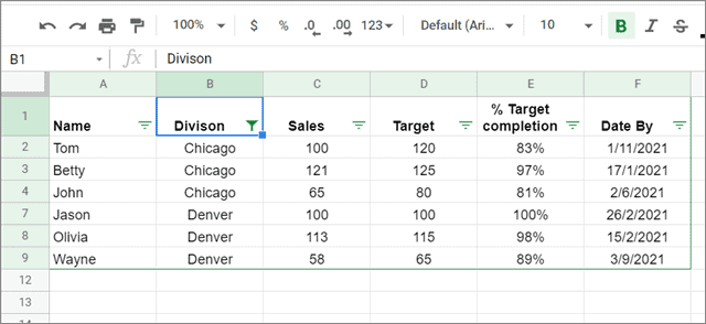
You can see the result after you click OK.

Remember that conditional filtering uses logical operators while value filtering focuses on a specific value in a given column.

Filter By Color

If you have done conditional formatting in Google Sheets and have colored cells, you can filter in Google Sheets by color.

For instance, let’s take the same sales sheet with colors as shown in the figure below.

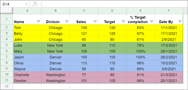
Now, the condition is to narrow down the data only to the sales figures in the New York division. So, you need to eliminate the remaining three divisions from column B based on their colors.

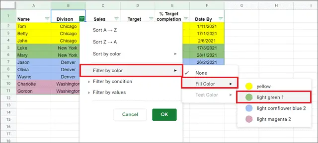
Open the Filter arrow from the header row and choose Filter by color. Next, select Fill Color and choose the color that represents the column conditions and data. Here, we have selected light green 1 as it represents New York.

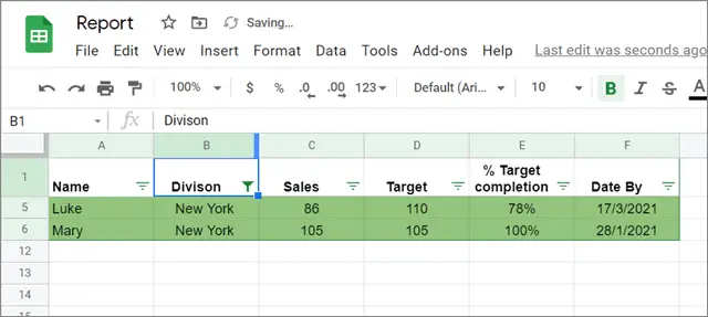
You can see the result once you select the preferences and click on OK. Only the data from New York will be visible because we have selected the corresponding color.

If you have colored text instead of colored cells, you can choose the Fill Color option and filter data accordingly.

Users also need to keep in mind that they can filter in Google Sheets using only one color at a time.

Filtering data by colors may be challenging if you are using too many colors in a datasheet. So, make sure you know the resource types, fields, and the colors they are represented by. Then, you can quickly filter the data based on colors.

How To Turn Off Google Sheets Filter

We learned how to filter in Google Sheets in two different ways in the previous method. Now, let’s take a look at how to turn off the Google Sheets filter in a straightforward step.

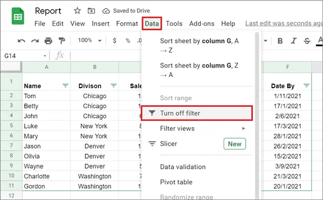
Navigate to the menu bar and click on the Data tab. Next, click on the ‘Turn off filter’ option.

You can also use the filter shortcut from the toolbar to turn it off. Once you do this, the original data will be visible. However, you will lose any unsaved filters after this process.

How To Save Filter Views

We have seen how to filter in Google Sheets and close the Google Sheets filter. If you are using a particular filter, you can also save it for future use.

Go to the Data tab and choose Filter views from the drop-down list of options. Then, select ‘Save as filter view’ from the nested menu.

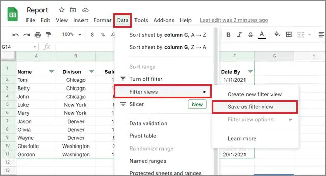
Once the new filter view is saved, you can give it a name to access it later.

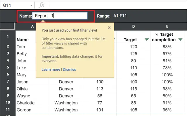
If you have shared this Google spreadsheet with other collaborators, they can also access your filters in this manner. In addition, you can save multiple filter views using this process.

How To Share A Filter View

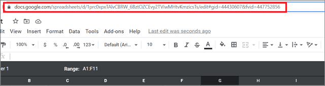
Sharing a filter view in Google Sheets is a cakewalk. All you need to do is copy the URL of the filter view and send it to the collaborators for accessing the filter view sheet.

Notice the &fvid=######## part at the end of the URL. This is a unique ID that allows you to share unique Filter View links with all collaborators.

Users can either grant editing permissions or only viewing rights to other collaborators. If a collaborator has permission to edit, all the edits are saved, and the changes may be applied to all collaborators.

If a collaborator only has viewing privileges, they can filter or sort data, but the changes will be only visible to them. With viewing rights, they can create a temporary filter for themselves. The original filter view remains unchanged. Apart from the filter feature, you can use a pivot table to summarize data according to your requirements.

How To Filter In Google Sheets On Smartphones

If you don’t have a PC available, you can use the filter function on the Google Sheets mobile app that can be used on tablets and smartphones.

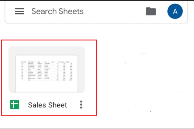
To begin with, open the Google Sheets mobile app and tap on the sheet in which you wish to add the filter.

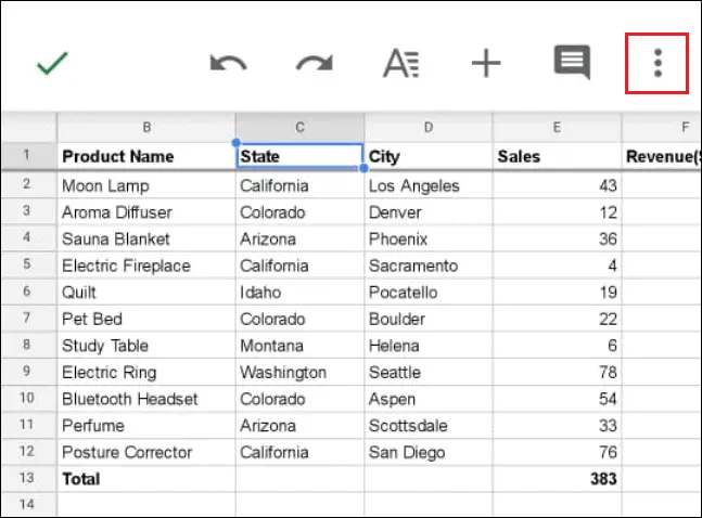
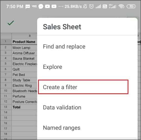
Now, select the column over which you wish to add the filter. Then, tap on the three vertical dots in the top right corner.

From the menu, select Create a filter.

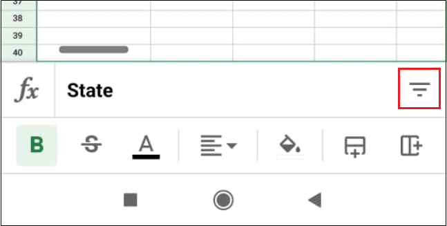
Now, move to the bottom of the screen and you will see the name of the column on which the filter has been added. Next, tap on the filter sign (three horizontal bars) to open the filtering options.

From here onwards, you can filter the data in the same manner as we did on PC. Here, we have filtered the data based on value.

That’s all about how to filter the data based on mobile. However, for better visualization purposes, we recommend that you use a PC while using the Google Sheets filter in a smartphone.

Conclusion

Data organization and its complex queries is a crucial aspect of managing large chunks of data. Before using a dataset for analysis, it is essential to arrange and organize the data for better comprehension. Google Sheets filter offers multiple features, functions, and filter operators for those who wish to manage their datasheets neatly.

If you wish to look at a limited chunk of data in a large datasheet, you need to know how to filter in Google Sheets. You can either save a filtered view for other collaborators to view the data or apply a filter to organize a dataset accordingly. Also, data filtering cannot be done in Google Docs; it is only possible in Google Sheets.