We use Google Sheets to store different types of datasets for multiple purposes. There may be instances where you need to access data in a different Google Sheets file. In that case, you need to know how to reference another sheet in Google Sheets to pull the required data.
To better understand, let me give you an example. Let’s say you have two spreadsheets in different files. The first Google spreadsheet contains the names of customers and the prices of the items they bought. The second sheet contains only the total amount spent by each customer. If you need to see how much each customer has spent, you need to reference the second sheet in the first one. If you have the reference data in the same file, you can know how to link cells in Google Sheets and refer to the data.
How To Reference Another Sheet In Google Sheets And Pull Data With Ease
Let’s look at the quick steps to pull the data and reference another sheet in google sheets for better and convenient reading.
How To Reference Another Sheet In Google Sheets
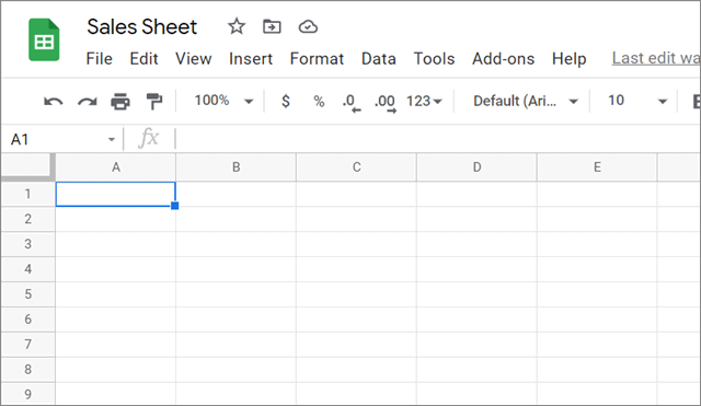
1. Open Google Sheets.
2. Select the cell in which you want to pull the data.
3. Enter the referencing Google Sheets formula.
4. Pull the data in the selected cell.
Note: The basic steps above will give you an idea of how the process is carried out. Now, let’s take an in-depth look at each step with detailed images.
How To Pull Data From A Spreadsheet In The Same Document
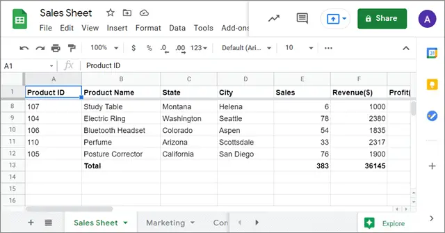
To reference another sheet in Google Sheets, you need to open both the spreadsheets that will be involved in this task. Then, make sure the data you want to pull into your spreadsheet exists in the same document. In the example given below, we will try to pull data from the Sales Sheet in the Marketing sheet.
The Sales Sheet will be our primary source sheet, and the Marketing sheet will be the destination sheet. Make sure you have proper sheet names for the spreadsheets you are working on.
To begin with, go to the destination sheet and select the cell in which you want to pull the data. This is where you will reference another sheet in Google Sheets. Here, we have selected cell A1.
Next, enter the formula in the correct syntax given below.
=<SheetName>!cell numberIn our case, we wish to pull the first four products from Sales Sheet to Marketing. So, the formula in the cell will be:
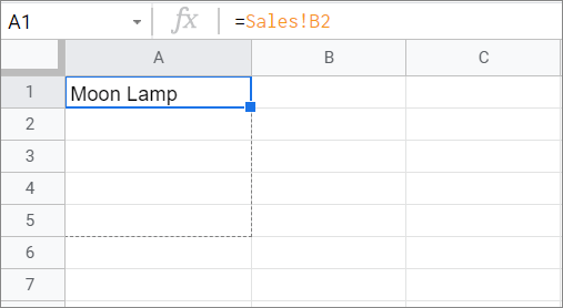
=Sales!B2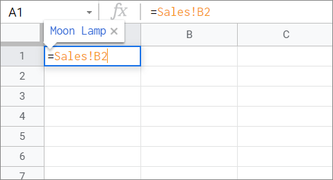
Make sure you mention the original sheet name only before the exclamation mark and not after it.
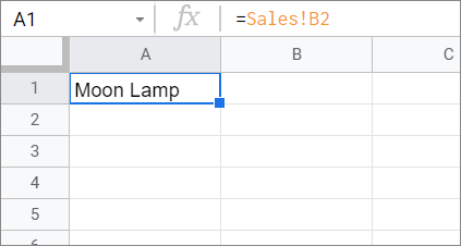
By doing this step, the data from source cell B2 in the Sales sheet will be pulled into the Marketing sheet.
We have seen how you can reference data from a single cell in another sheet. But, what if you want to import a range of cells from the original spreadsheet file? Well, the answer is to use the fill-down method in Google Sheets.
All you need to do is hover the cursor over the cell where you have pulled the data. Then, when the ‘+’ sign appears, drag it down to a select number of rows until which you want to import the data from the primary sheet.
In the image below, you can see a dotted border that represents the selection of rows in which you want to pull data from multiple cells.
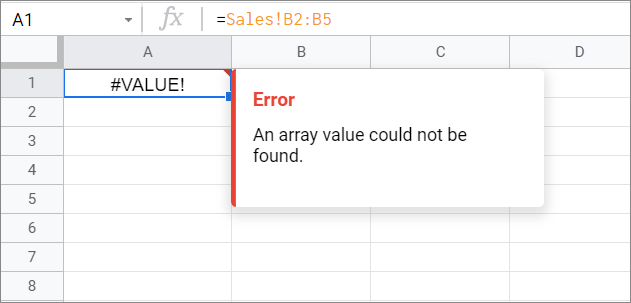
One essential thing to understand here is that you cannot use a range of cells in the referencing formula. For instance, if we enter the formula Sales!B2:B5 in the selected cell, it would give a #VALUE error as shown below.
So, the best method is to reference data using a single cell and then use the fill-down method to import the remaining range of data from the primary sheet. If the data is large and you want to retrieve precise information from it, use the query function in Google Sheets.
How To Pull Data From A Spreadsheet In A Different Document
Sometimes, you may need to source data from a different sheet in a different workbook altogether. In such cases, you can use the IMPORTRANGE function to reference another sheet in Google Sheets.
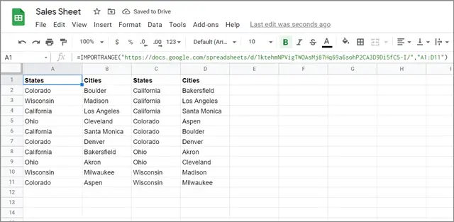
In the example given below, we will try to import data from the S&C sheet to the Marketing sheet. Both spreadsheets are part of different Google Sheets documents. The S&C sheet will be our primary source sheet, and the Marketing sheet will be our destination sheet.
To start with, select the cell in the Marketing sheet where you want to import the data from the S&C sheet.
Next, enter the IMPORTRANGE formula in the selected individual cell of a column. The syntax for this function is –
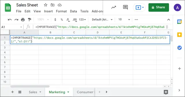
IMPORTRANGE("<URL>" , "<CellRange>")So, the formula in our case will be as given below. Also, it’s better to enter this formula in the formula bar instead of the cell.
When you copy and paste the entire document URL hyperlink, make sure you highlight and copy the URL only upto the ‘/’ mark. This is how the custom function will look once you have added the details.
IMPORTRANGE(“https://docs.google.com/spreadsheets/d/1ktehmNPVigTWOAsMj87Hq69a6sohP2CA3D9Di5fC5-I/”, “A1:D11”)
Note: The doc link given above is used as an example. It is not meant to be accessed by users.
You need to insert the single spreadsheet URL of the source worksheet in the formula.
If you have more than one sheet in the document you are exporting from, you need to mention the sheet tab name. Then the range will look like ‘Sheet2!A1:D11’ instead.
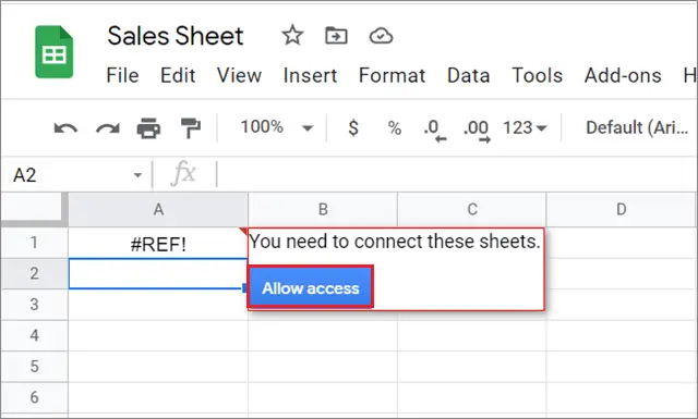
When you hit the Enter key after entering the formula, you will get a #REF error. Google Sheets will show you an ‘Allow Access’ button asking permission to connect the two sheets. Click on the button to grant access and view the result.
Once you allow the access, this is how the sheet will look like.
Compared to the previous method, one good thing is that you can enter an entire cell range in the formula and import it from another spreadsheet file. Here, you don’t need to use the fill-down method as you can specify the data range you want to import in the formula itself. In this manner, you can pull data from multiple sheets.
How To Add Data From Multiple Sheets In A Different Sheet
Now, let’s look at how we can compile data stored in different sheets in a separate sheet in the same document.
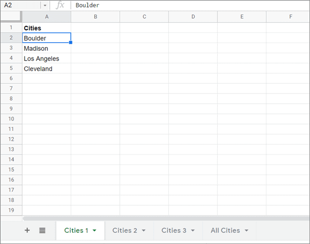
Here, we have three sheets viz., Cities 1, Cities 2, and Cities 3. The aim is to compile all the data in these sheets and pull it into the ‘All Cities’ sheet.
To begin with, go to the destination sheet, i.e., All Cities, and enter the formula given below.
{
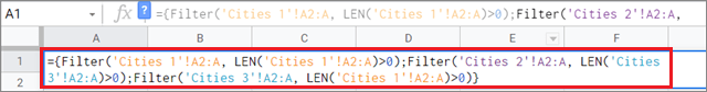
=Filter('Cities 1'!A2:A, LEN('Cities 1'!A2:A)>0);
=Filter('Cities 2'!A2:A, LEN('Cities 2'!A2:A)>0);
=Filter('Cities 3'!A2:A, LEN('Cities 3'!A2:A)>0)
}
FILTER(‘Cities 1’!A2:A, LEN(‘Cities 1’!A2:A)> 0) – this expression means the data from column A of the “Cities 1” is considered, excluding the values that are equal or less than 0.
This is how the Filter function will look.
Press Enter after you have entered the formula. This is how the result will look after the function is executed.
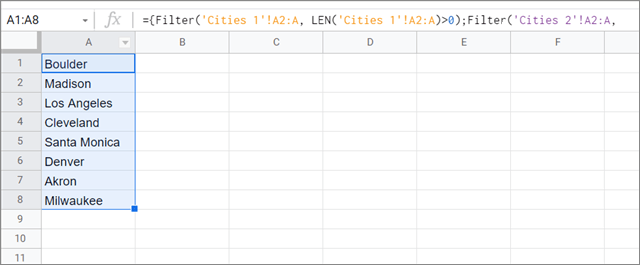
That’s all about referencing data from different sheets into a single column.
How To Look Up Data Using The VLOOKUP Function
If you have stored related data in multiple sheets in the same document, you may need to look up the data from the current sheet while using the other sheet as an absolute reference.
For instance, let’s say Sheet1 contains employee names and their respective roles. Sheet2 contains employee names and salaries. Now, the task is to find out the top three roles that draw the highest salaries in the organization.
Here, you need to look up the data in one sheet while using another sheet as a relative reference to conclude. You can do this task if you know how to use the VLOOKUP function in Google Sheets.
Conclusion
Data referencing is the need of the hour if you have stored large chunks of relational data in different spreadsheets in the same or multiple worksheets. So, if you know how to reference another sheet in Google Sheets, it will increase your productivity. It will be easy to read data between two different sheets in different tabs.
Pulling data allows users to save that hassle and derive meaningful insights out of it. You can use any of the methods mentioned above, depending upon the situation you are in. You can also cell reference data from another sheet on mobile. You need to follow similar steps as to what we saw in the PC method and calculate results on the Google Sheets mobile app.
FAQ
How do I link data from one Google spreadsheet to another?
You can use the cell reference formula or the IMPORTRANGE function to link data from different sources.
Can I reference a cell in another Google sheet?
Yes, you can reference a cell in another Google sheet.
How do I reference another sheet?
Click the cell in which you want to enter the formula. Enter the formula =<SheetName>!cell number. Press Enter key to import the data.


