Google Sheets offers numerous ways to sort and filter data so that users can check specific entries according to their needs. One such feature is the pivot table. It allows you to isolate a large datasheet. Then, a specific data slicer in Google Sheets or Excel sheet filters these pivot tables and charts to create an interactive report or dashboard.
However, before we get on with this exercise, it is essential to know how to create charts and a pivot table in Google Sheets. Adding a slicer is useful when you need to hide entries that do not match specific predefined filter criteria. In all, slicers allow users to organize data better and improve pivot tables and charts.
How To Use Slicer In Google Sheets
A slicer floats above the data and can be used to filter multiple columns at once. Since it isn’t fixed to any cell, you can move and align it as per your requirements. Using Google Sheets slicers isn’t a cakewalk; you need to practice it regularly to get good at it. Let’s take a peek at how to use slicers to enhance data visualization.
How To Use Slicer In Google Sheets
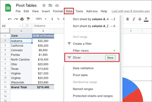
1. Open a Google spreadsheet.
2. Click on the Data tab and select slicer.
3. Specify the Data range and Column to filter in the right sidebar.
Note: These are the basic steps that can help you throughout the process of creating a slicer. Now, let’s look at how to use slicer in a Google sheet.
Details For Using Google Sheets Slicer
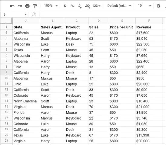
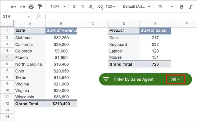
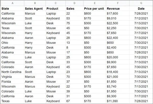
Let’s consider the sample sales sheet given below. This is a record of a company named Simson’s International that has deployed five sales agents to sell their products in the USA. The first row is used as the row header in the document.
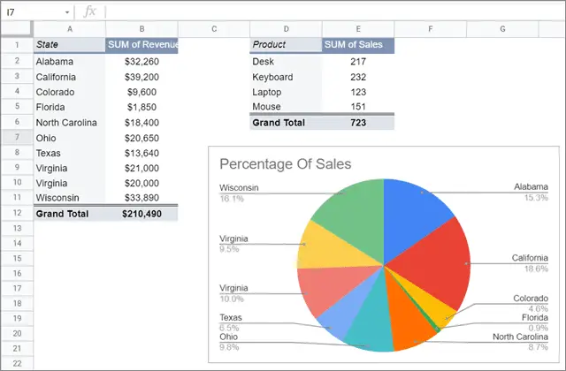
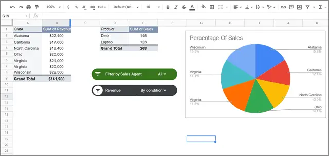
Next, we have two pivot tables and a pie chart. The first Google Sheets pivot table displays the total revenue generated in each state, while the second indicates the total sales made by each sales agent. The pie chart displays the percentage of sales made in each state.
We aim to slice and dice data to obtain a filter view using the slicer in Google Sheets.
Create A Slicer Based On A Column
This step will aim to filter the first pivot table, i.e., the sales and revenue table, based on sales agents.
To begin with, select the entity in question. Here, we will select the sales and revenue pivot table. You can click on any cell in the table, and it will be selected.
Navigate to the menu bar and click on the Data tab. Then, select slicer from the drop-down menu.
You will see the black slicer bar once you complete this step.
When you click on the three vertical dots on the slicer in Google Sheets, select the Edit slicer option to open the right sidebar for editing the options.
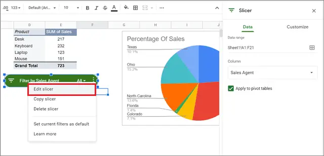
From the right sidebar, you can start customizing the slicer as per your preference.
Customizing The Slicer
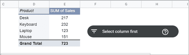
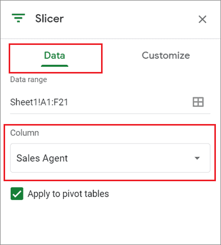
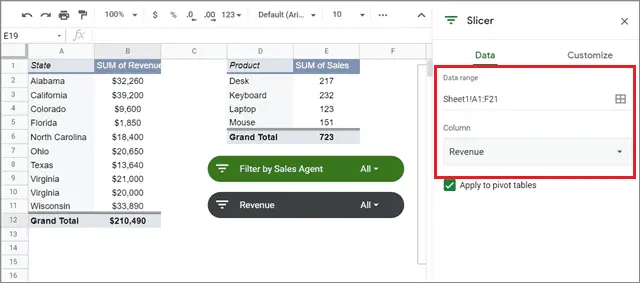
If you need to customize the slicer, you need to select the column you want the slicer to filter. In this example, we will filter the data according to the Sales Agent column.
So, select that column in the Data tab of the slicer sidebar. The data range Sheet1!A1:F21 specifies that we have used Sheet1 as the source sheet for data analysis.
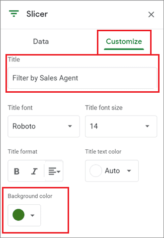
If you don’t like the color, you can change it from the Customize tab in the slicer settings sidebar. Here, we have changed the background color and slicer title.
Once you do these settings, you can now play around with the slicer in Google Sheets.
Use Slicer To Filter Data By Value
Note: We had already established earlier that we will filter the data based on the Sales Agent column. Accordingly, we have also selected the column in the Data tab in the slicer sidebar.
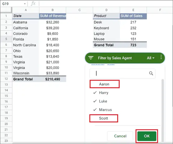
Let’s see how to use the slicer to filter the data. The condition is to see the total sales made by Marcus, Luke, and Harry combined. This means we will be leaving Aaron and Scott out of the equation.
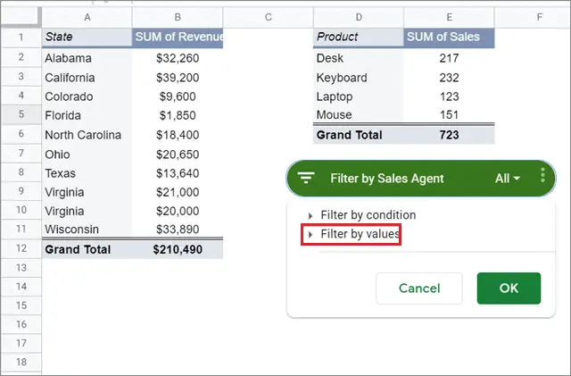
To begin with, click on the ‘All’ drop-down arrow on the slicer.
This will show two filter options: Filter by condition and Filter by value. In our case, we need to filter the data based on value.
We have unchecked Aaron and Scott from the list to satisfy the condition we have established above. Once you filter data as per your preferences, click on OK to obtain the result.
Notice that the grand total for both the pivot tables has decreased, and the pie chart also looks different from what we saw earlier.

This is how the result will look after you use the slicer in Google Sheets to filter the values.
Use Slicer To Filter Data By Condition
Let’s say you want to find out all the states that have made more than $15000 in revenue from the example above. We can create a separate Google Sheets slicer for this purpose. Follow the same process to create one, as we saw in the previous example.
Here, we need to specify the condition to execute the operation. Since we need to consider revenue as the decisive factor, we have specified the same in the Column section of the slicer sidebar, as shown below.
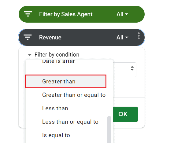
Click on the All menu in the slicer and select Filter by condition.
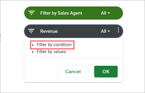
Specify the condition you want to execute on the data. Here, we will choose the Greater than option as we need to see the states with revenue of greater than $15,000.
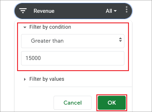
Next, enter the threshold based on which you wish to sort the data. Here, we will enter 15000. Make sure you don’t enter any other symbol when you’re working with numbers. For instance, if we insert $15000 here, Google Sheets would return an error.
Press OK after you have specified the details in the slicer in Google Sheets.
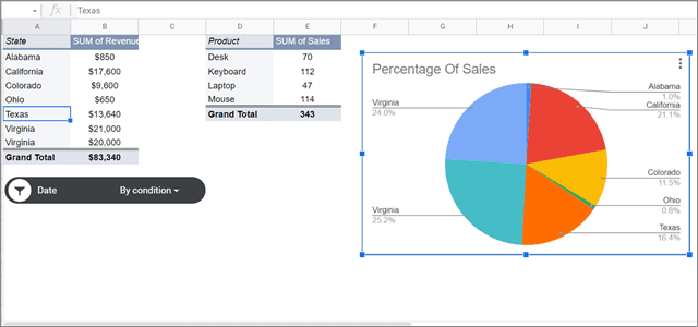
You will instantly see the filtered result that shows the number of states that have garnered revenue greater than the specified amount.
Interestingly, you can also see that the second pivot table is also affected by the condition. It shows the products that have made more than $15,000 in sales, albeit the actual amount isn’t visible. This tells us that a slicer in Google Sheets can control all the variables at once.
Users can filter data in pivot tables based on certain conditions related to date and text. You can also add your custom formula for filtering the data based on custom conditions.
How To Use Slicer Based On Dates
We have seen how the slicer can filter data based on value and condition in the previous example. You can also use the slicer in Google Sheets to filter the pivot table results based on dates.
Here, we have added a Dates column to make things clearer.
Note: When you add a new column to the original table, make sure you update the data range for the pivot tables as well. If you carry on with the operations without updating the data range, you will face the #REF error.
Now, let’s say you have to filter the pivot tables to obtain sales figures registered only after 17th July 2021. You can filter data by value or condition depending on your choice.
However, filtering by condition makes more sense in this case as there will be less work involved. If you choose to filter by value, then you need to manually cancel out all the dates that occur before the specified date.
Create a slicer based on the Date column and enter the condition as shown below.
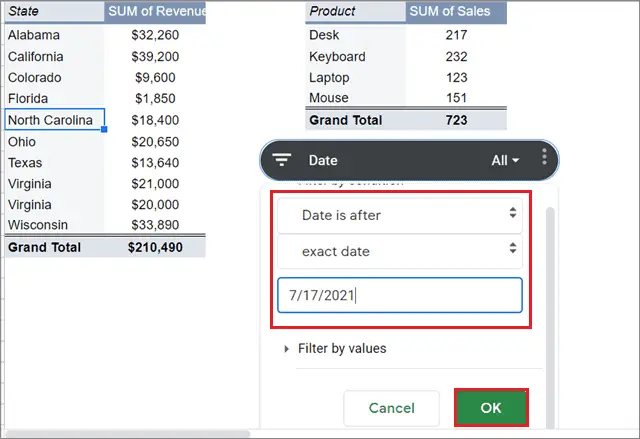
Once you press OK, you can see that the pivot tables and the pie chart will be filtered according to the given condition.
That’s all about using the Google Sheets slicer for slicing and dicing data based on dates.
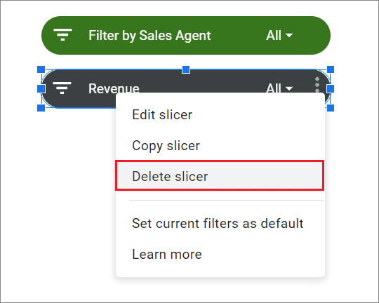
How To Delete A Slicer In Google Sheets
Deleting a slicer is a simple task. All you need to do is click on the three vertical dots in the slicer bar and choose Delete slicer from the drop-down menu options.
That’s pretty much everything about how to use a Google Sheets slicer. However, if you want to keep a slicer for the long term, you can choose ‘Set current filters as default’ from the below drop-down menu. This will make your current filter charts permanent, and they will be visible to all the collaborators on the document.
Once you have filtered the data correctly, you can use conditional formatting in Google Sheets to make the data easily readable. You can also use the data validation feature if you wish to add drop-down lists to a filled or blank cell in a spreadsheet.
The Difference Between Slicer And Filter
The primary function of a slicer and the Filter formula or feature is the same: to filter data in a spreadsheet. However, some of the common differences are that slicers help in better visualization of data than filters.
Since it’s a visual element, you can position slicers anywhere in the spreadsheet, something that cannot be done with filters. Overall, filters are used to filter column data in a very basic manner in the spreadsheet. Slicers, however, serve the more advanced purpose of filtering data in pivot tables and charts.
Conclusion
Making a slicer in Google Sheets might seem to be a complex process, but once you get the hang of how it is used, filtering data will be a cinch for you in Google Sheets. Using a slicer is similar to using the filter feature or filter function to obtain specific data from a large dataset. In fact, you can use a slicer instead of the filter feature to play around with the primary data.
However, slicers are more useful when you want to filter pivot tables. Slicers can control multiple charts and pivot tables at once. This affords users the power to control multiple variables based on a condition or a value in Google Sheets. Also, it is essential to remember that slicers apply only to an active sheet. You can apply multiple slicers to filter a single dataset by different columns. Also, users cannot create a slicer in Google Sheets mobile app. That functionality can be availed of only on the PC.
FAQs
What does the slicer do in Google Sheets?
A slicer comes in handy in filtering data in pivot tables and charts in a Google spreadsheet.
How do you use a Slicer in Google Sheets?
Go to the Data tab in the spreadsheet and click on slicer from the drop-down list of options to use a slicer.
How do I lock a slicer in Google Sheets?
Unfortunately, there is no way to lock a Google Sheets slicer. However, you have that facility at your disposal if you are working with the Microsoft Excel slicer.
Is there a shortcut to create a slicer in Google Sheets or Excel file?
No, there is no shortcut for creating a slicer in a Google sheet or an Excel worksheet.


