When it comes to project management, it’s nigh impossible to envision project execution without a Gantt chart in Google Sheets. Gantt charts were invented by Henry Gantt, an American mechanical engineer, in 1910. Ever since then, they have been widely considered as an essential project management tool.
Prior to execution, managers need to plan the number of project tasks and resources required to complete a project successfully. A Google Gantt chart helps map out all the tasks and resources and provides a bird’s eye view of how the project is functioning over a particular period. If you wish to map out your project tasks, you can create a timeline chart template for better management.
Pros and Cons of Gantt Charts
Like everything else, the Gantt chart in Google Sheets also has its pros and cons. To start with pros, you can easily get started with a Google Gantt chart using the stacked bar graph method in Google Sheets. You can also use ready-made Gantt chart templates if you don’t wish to create one manually.
Users can also share their Gantt charts with other people for collaboration. If you’re using a stacked bar chart type for your Gantt chart, you can even publish it on the Internet or download it as a PDF or PNG.
Coming to the cons, the Gantt chart in Google Sheets is not suitable for complex projects. If there is a list of tasks and resources involved, a Gantt chart may be insufficient to track all the activities. Since complex projects require more data, this can also make the performance slower.
Also, it’s challenging to define milestones in a Gantt chart clearly. If there are too many milestones, the best you can do is use different colors to group them.
Elements of Google Sheets Gantt Chart
There are five significant elements you need to know before creating a Google Gantt chart.
1. Tasks: Tasks are situated in the left column of the Gantt chart sheet. You can group these tasks according to their categories.
2. Timeline: The timeline is displayed on the horizontal axis at the top. The scale can be yearly, monthly, weekly, or daily.
3. Bars: Bars are used to indicate the task duration. They also let users know how many critical tasks are running simultaneously in the entire project.
4. Milestones: Milestones can be used to divide a project into different phases. They are usually marked with diamonds.
5. Resources: Resources are people or tools required to complete the tasks. You can display the resources, but that can make your Gantt chart cluttered.
How To Create Gantt Chart In Google Sheets
Creating a Google Sheets Gantt chart can be intimidating for beginners. However, once you get the hang of it, you can quickly make Gantt charts for managing projects. If you do not favor creating one, you can use ready-made Gantt chart templates to plan your projects.
How To Make A Gantt Chart Using Stacked Bar Chart
You can make a Gantt chart in Google Sheets using the stacked bar chart with a simple step-by-step guide for your project plan.
1. Create The Data Sheet
To begin with, you need to create a data table containing the list of tasks and dates on a blank spreadsheet. If you use a project management software like JIRA or Asana, you can import this data from those tools into a Google spreadsheet.
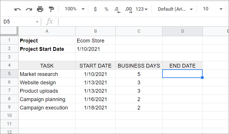
For this instance, we will be using this mock data of a project plan.
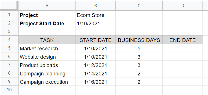
We have the start dates and the number of business days required to complete each task. Therefore, the first step is to calculate the end dates of each task.
However, the time constraints for each task also contain non-working days. We need to eliminate those days to get a precise and accurate estimate of the working days. This condition can be achieved using the WORKDAY function.
To begin with, enter the formula given below.
=WORKDAY(B5, C5 - 1)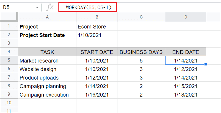
‘start’ is the start date of a task, and ‘days’ denotes the number of working days. We are subtracting 1 from days to eliminate the non-working days. This number depends on how many non-working days are in a week, month, or year.
Next, we need to calculate the number of calendar days required to complete a task. Enter the formula given below to calculate the calendar days.
=D5-B5+1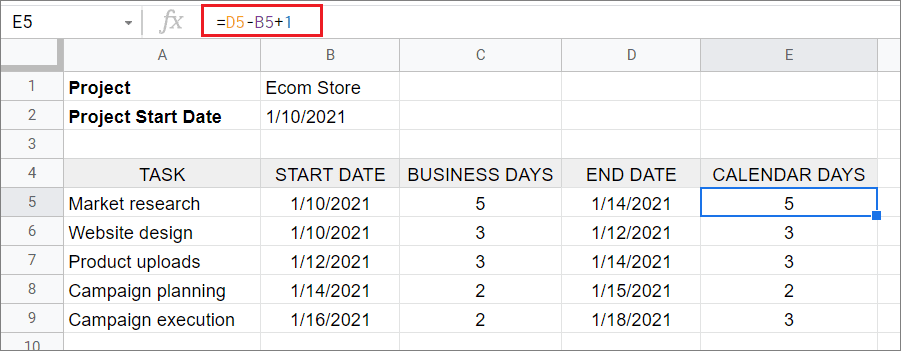
Your datasheet is now ready to be converted into a Google Gantt chart.
2. Format The Date Column
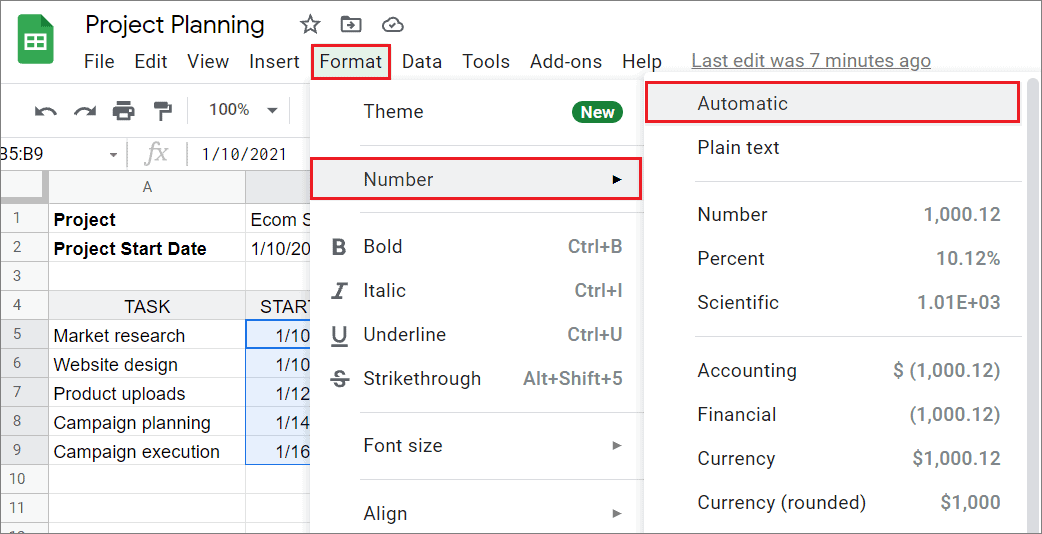
Once the Google sheet is ready, you need to insert the stacked bar chart to visualize your project schedule. Before that, you need to change the format of the start dates.
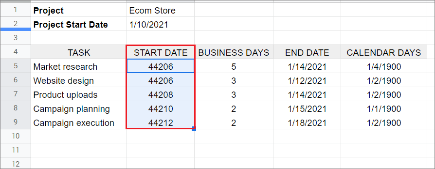
First and foremost, select the Start date column. Then, click on Format, choose Number, and select Automatic.
This is how the Start date column will look after you format it.
3. Insert A Stacked Bar Chart
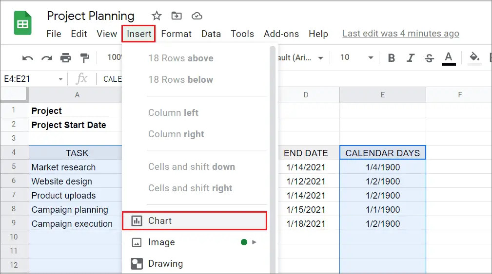
To insert the stacked bar chart, first highlight the Start, Task, and Calendar Days columns. Then, click on Insert and choose Chart.
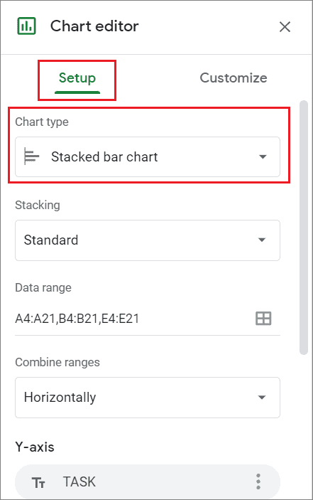
In the Chart editor sidebar, select Stacked bar chart.
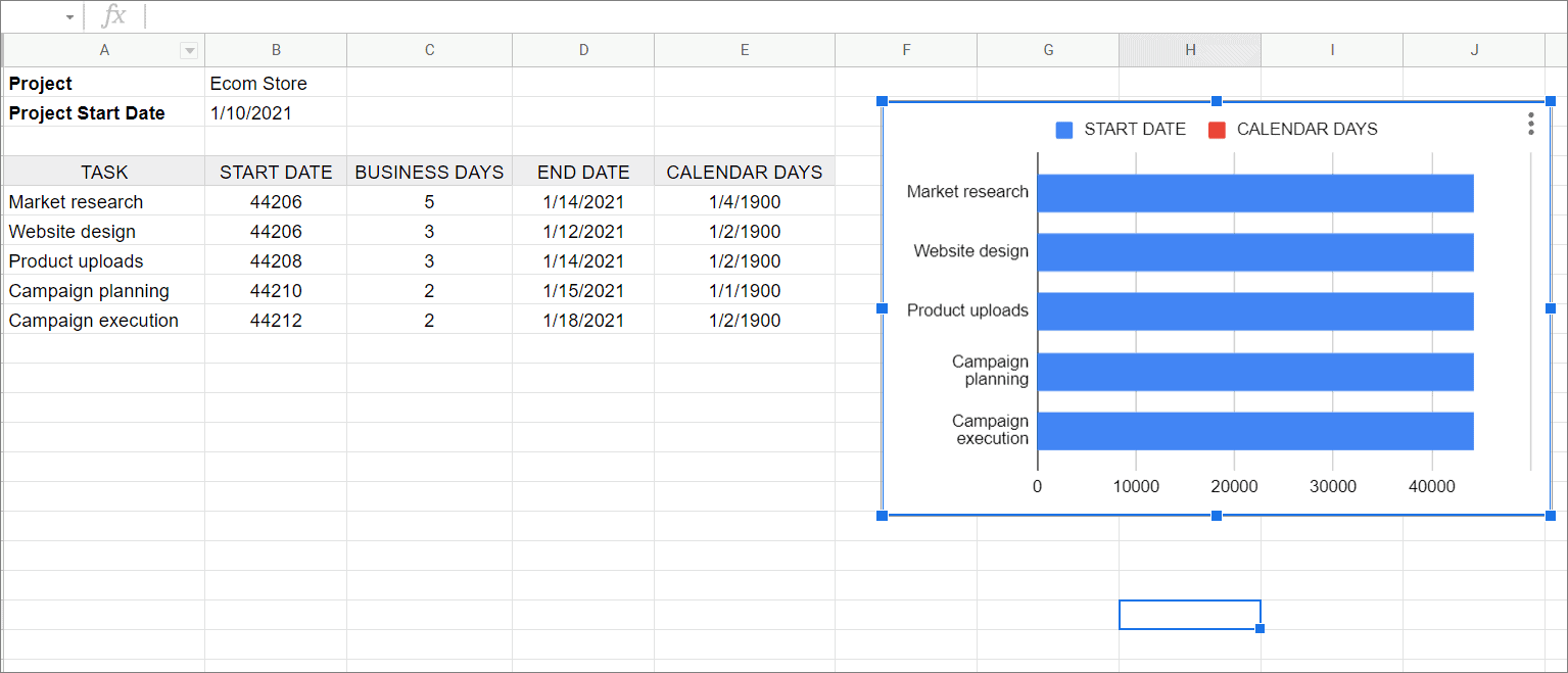
This is how the Gantt chart will look in the spreadsheet.
4. Customize The Date
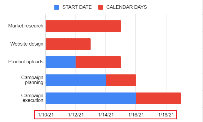
Now, let’s customize the chart’s horizontal axis to show proper dates instead of numbers. We’ll also customize the bars’ colors.
In the Chart editor, click the Customize tab and expand the Horizontal axis section. Next, change the Min value to 44206, which is the start date of the first task.
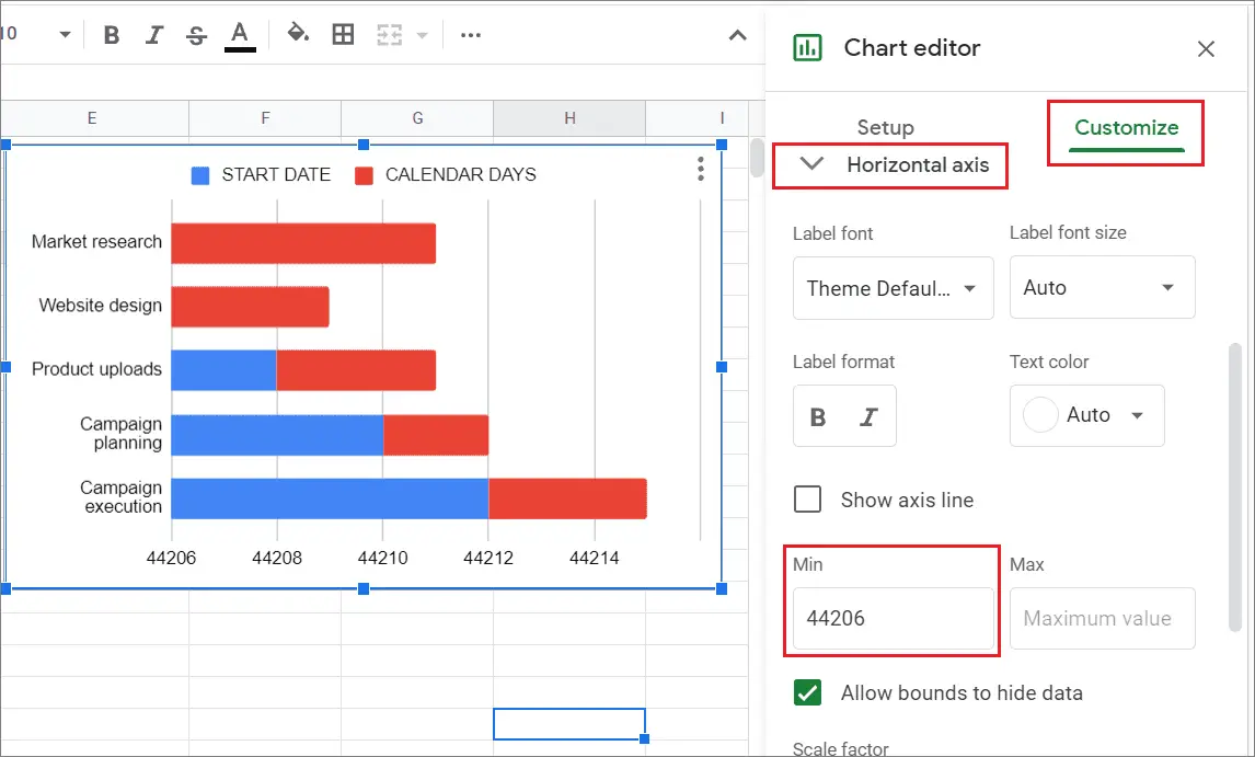
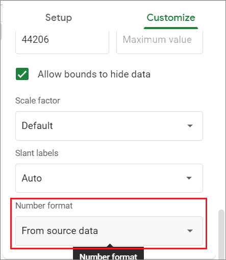
Then, scroll down to the Number format section and click on it.
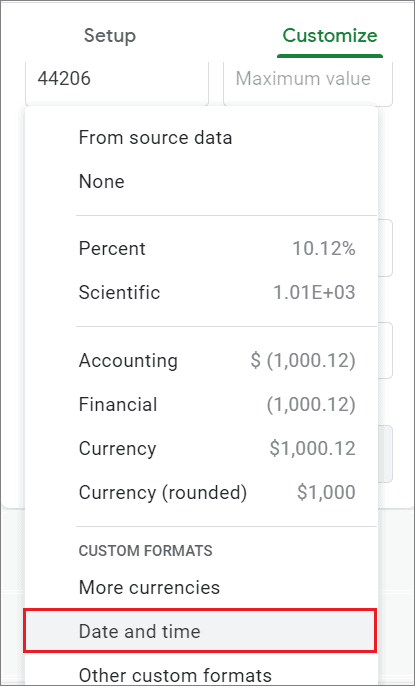
Choose Date and time from the drop-down options.
Select the date format and click on the Apply button.
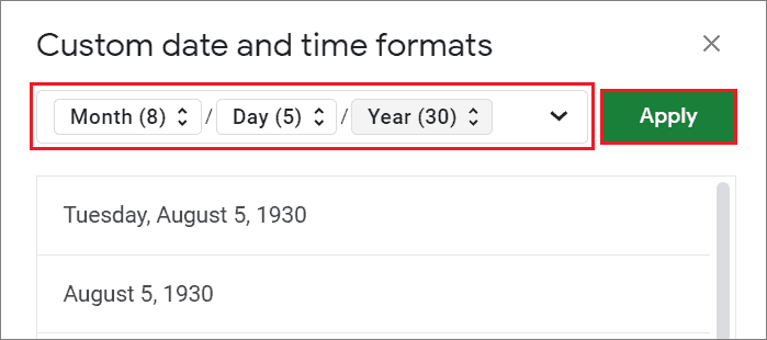
Notice that your X-axis now displays dates instead of numbers.
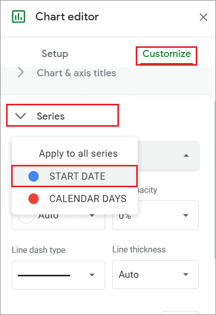
5. Customize The Bars
To customize the bars, expand Series and select the START DATE option from the dropdown menu.
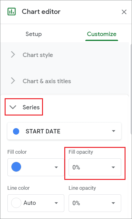
Change the Fill Opacity to 0%.
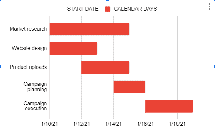
Notice that your chart looks more like a basic Gantt chart instead of a standard stacked bar chart.
If you like, you can also customize other things using the Chart editor. For example, you can modify the chart’s title, legend, bar color, slant labels, and so on.
Finally, make sure you change the formatting of the Start date column and bring it back to the previous state. Select the Start date column, click on Format, choose Number, and select Date and time from the drop-down menu options.
How To Make A Gantt Chart Using Conditional Formatting
If you are well aware of performing conditional formatting in Google Sheets, you can quickly whip up a Gantt chart in Google Sheets within minutes on a spreadsheet. The whole process comprises seven steps.
1. Prepare The Chart With Tasks And Dates
Similar to what we did in the previous method, you need to prepare a chart showing details of the project in a Google spreadsheet, as shown below.
The project sheet should consist of four columns: Task, Start, Days, End date.
In the previous example, we exclude weekends from the End date column. If you want to include them, enter the spreadsheet formula given below.
=B5+C5-1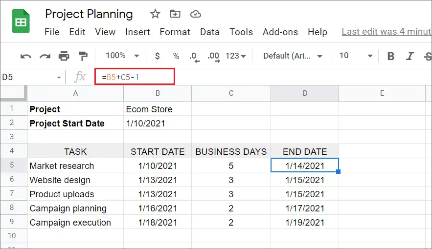
Once you get the result in one cell, you can use the auto-fill feature in Google Sheets to generate the result for other cells.
2. Create Task Dependencies
In most cases, we come across dependent tasks. This is a condition where a task cannot start unless the previous project task is completed.
To tackle this situation, you need to create task dependencies between tasks in a Gantt chart in Google Sheets.
In this example, let’s create interdependency between the first two essential tasks, i.e., Market research and Web design. You need to have the End dates for this purpose. The primary aim is to start the Web design task only after the Market research task is over.
Enter the following spreadsheet formula in cell B6.
=D5+1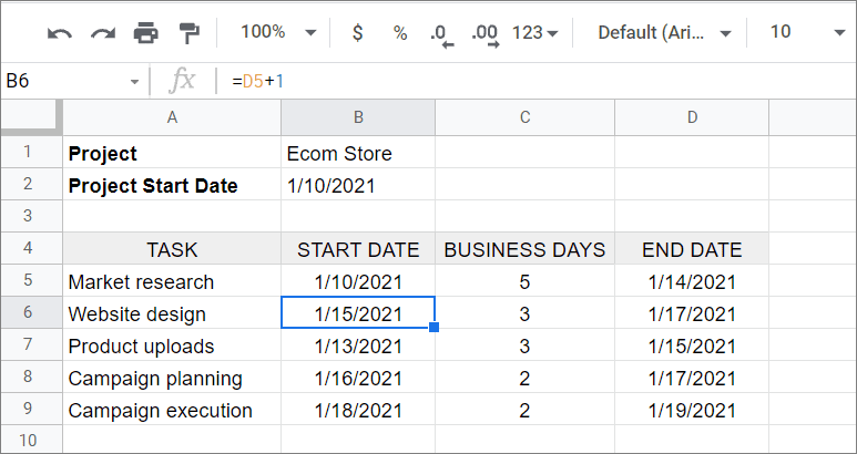
The B6 cell contains the start date of the Website design task. The entered formula will ensure that Web design starts only on the day after Market research is complete.
If there is a delay in finishing Market research, the start date for Web design will be automatically delayed due to this formula.
In this manner, you can create dependencies for multiple tasks.
3. Create The Timeline
To create a timeline for a Gantt chart in Google Sheets, first, you need to do some fundamental formatting changes to the cells.
We will create a two-week timeline in this example.
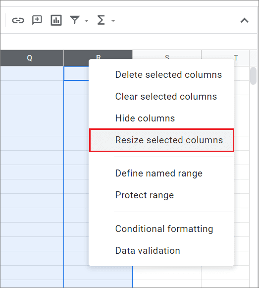
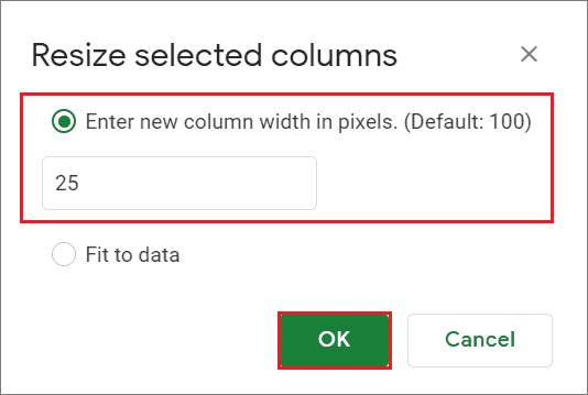
To begin with, we will first change the cell size of all the columns from E to R. To resize the columns, select and right-click on them. Then, choose – Resize Columns E – R from the context menu.
Next, set the width of each column to 25 pixels in the column size dialog box and click OK.
Now, let’s resize the blank third row. Select the entire row and right-click on it.
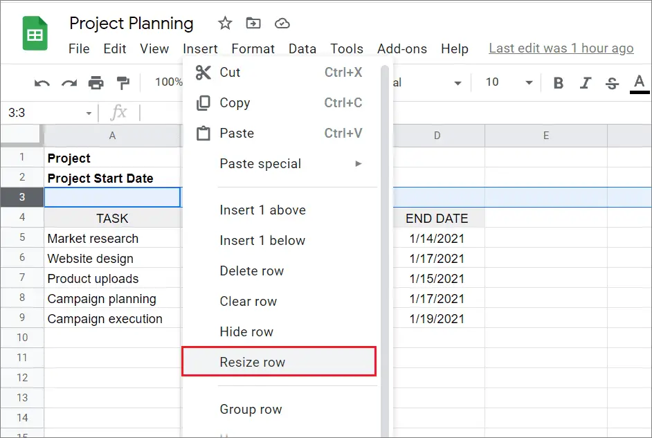
Then, set the height of the row to 60 pixels in the small dialog box that appears. Click on OK after setting the pixels.
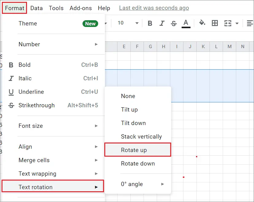
Now, you need to change the rotation of the third row.
To begin with, select the entire third row and click on the Format tab. Then, select Text rotation and choose Rotate up from the nested drop-down menu.
Now, enter the dates in the third row as shown below. To begin with, enter the project start date in cell E3 and drag it to cell R3.
In the row below the dates, you need to enter the first letter of each weekday to make sure the Google Sheet Gantt chart is more informative.
To do this, use the following formula.
=LEFT(TEXT(E3, "ddd"), 1)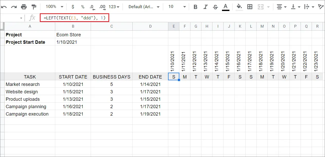
Once this formula is executed, use the fill-down method to fill up the remaining column cells. You can also color this entire row so that it’s easily distinguishable.
4. Add Bars Using Conditional Formatting
Bars are the heart and soul of a Gantt chart in Google Sheets. They are the graphical representation of blocks of time that present an overview of a task or an entire project.
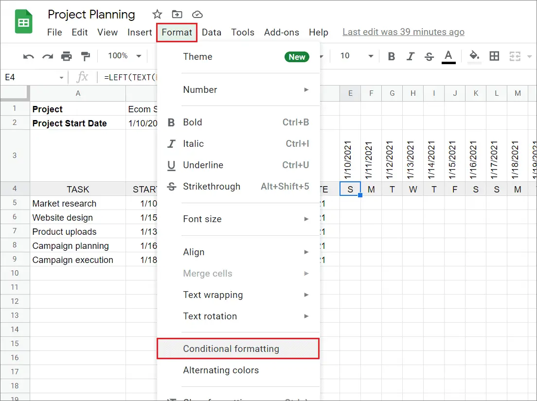
First and foremost, click on the Format tab and select Conditional formatting from the drop-down menu.
Then, enter E5:R10 in the Apply to range box. E5:R10 is the data range denoting the bars’ area.
Then, select Custom formula from the drop-down and enter the given formula in the text box.
=AND(E$3>=$B5,E$3<=$D5)This formula evaluates the dates that are between each task’s start date and end date to TRUE.
Then, you need to change the color of the cells that match the given condition.
To do this, go to the Formatting style section and click on the color bucket icon. Next, select a color of your choice. Here, we have chosen green.
This is how the final result will look.
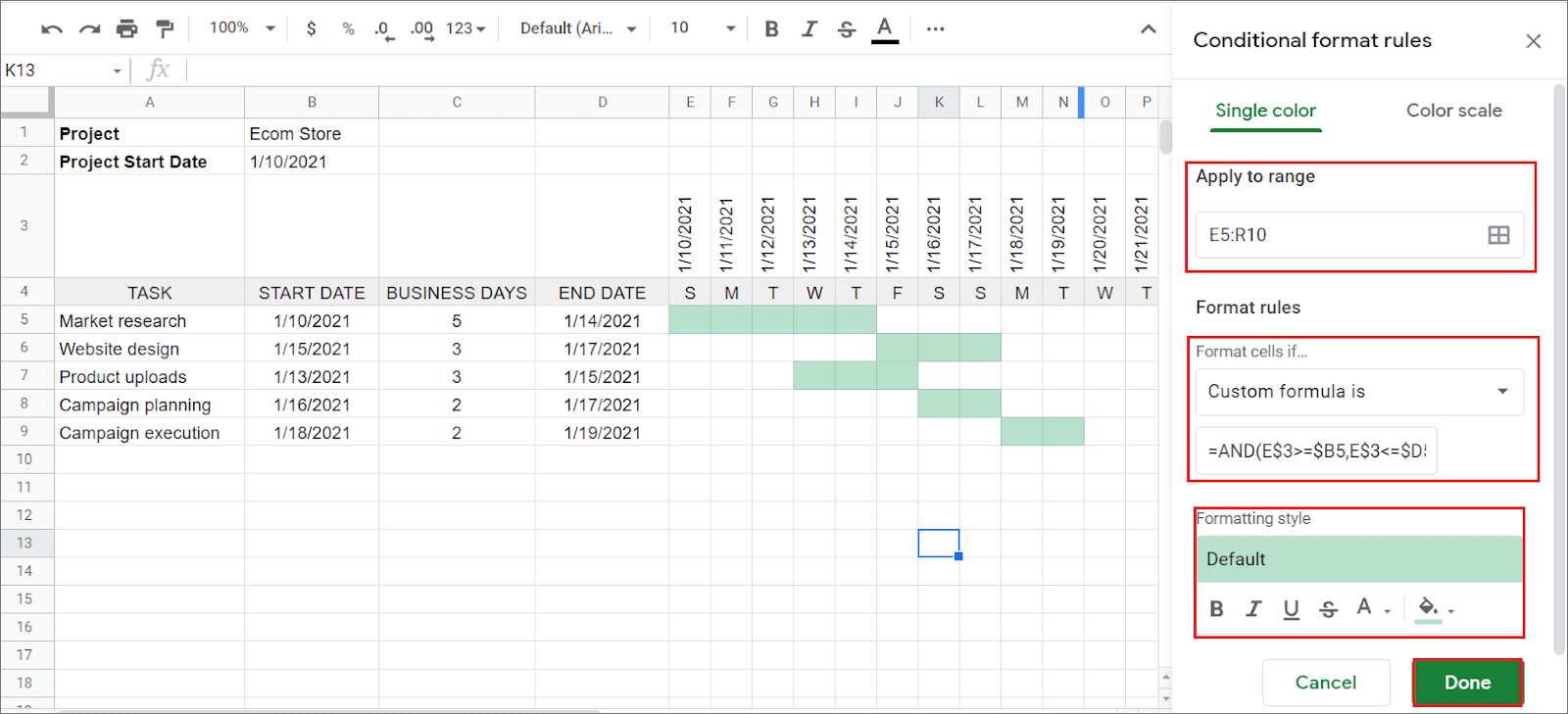
Click on Done in the bottom-right corner to close the conditional formatting sidebar once you have made all the settings.
5. Make A Dynamic Timeline
We have already seen the basic steps to create a Gantt chart in Google Sheets using conditional formatting rules.
Once you have created the basic chart, you can make your timeline dynamic. A dynamic timeline means whenever you change the project start date, the entire date range of your timeline should change automatically.
To do this, you need to link the first date of the timeline to the project start date.
Click on the first date cell(E3) and enter the formula as given below.
=B2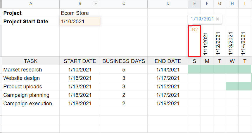
B2 contains the project start date. When you change this date, the first date of the project will change automatically.
Now, choose the second date cell(F3) and enter the formula as given below.
= E3+1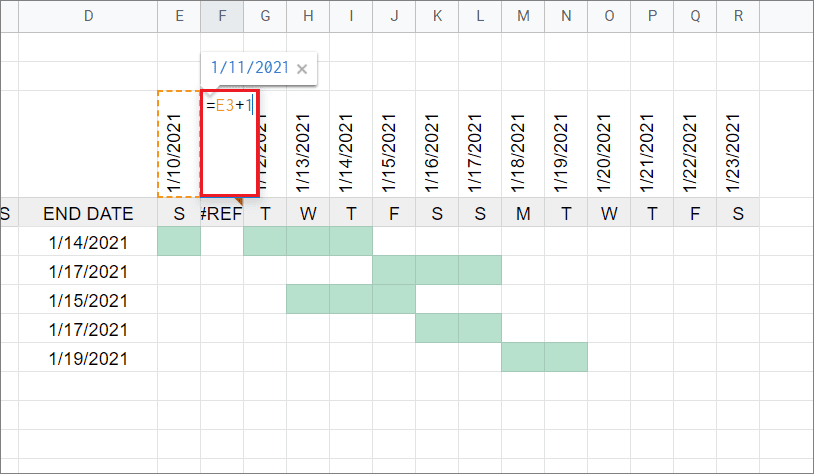
Now, drag the blue dot until R3 to add one day each to the next dates.
Once this step is done, your timeline will become dynamic. To test it, change the project start date and see how the results change.
6. Create A Progress Bar
A progress bar will give the users an idea regarding the amount of work done on a particular task.
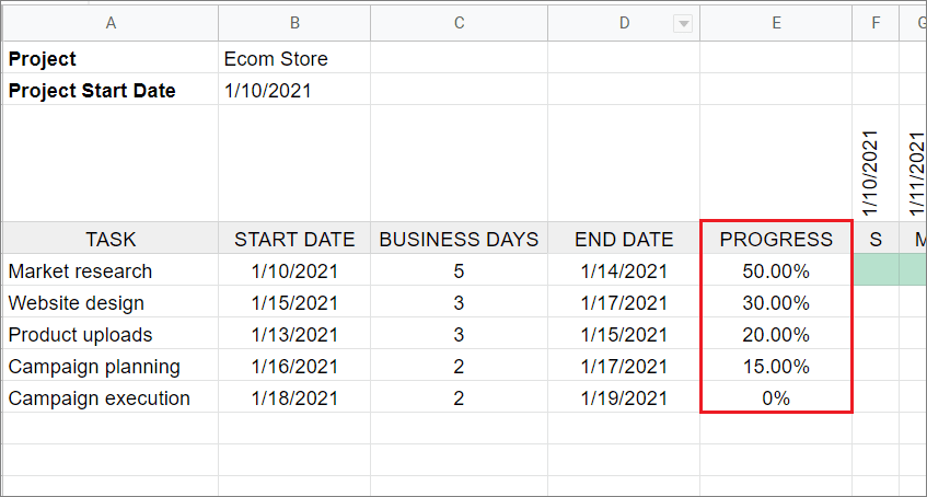
To begin with, add a new column called PROGRESS next to the END column. You need to use the percentage formatting for this column.
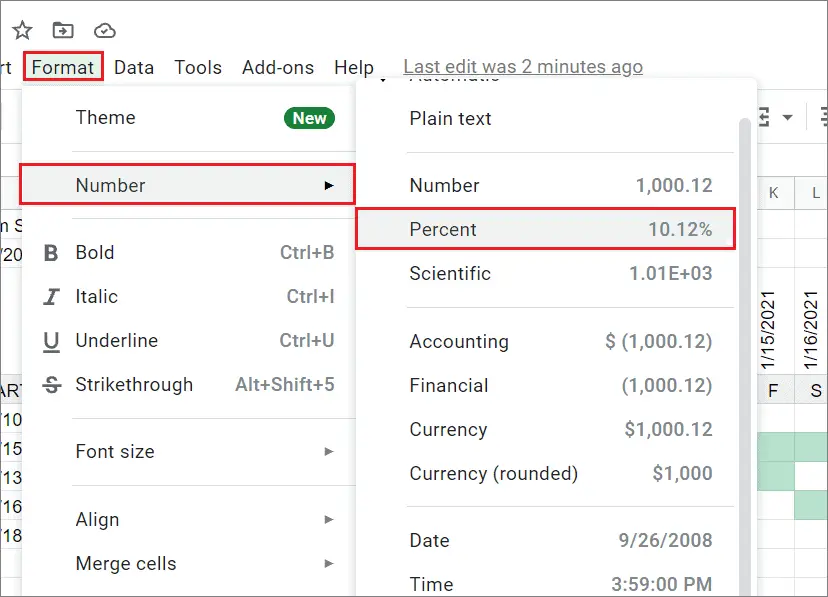
Select the column and click on the Format tab. Then, choose Number and select Percent from the menu.
Once the formatting is done, you can put values in this column.
Now, we need to create a graphical representation of the progress bar. Add another column next to the PROGRESS column.
Enter the given formula in the first cell of the newly created column.
=IFERROR(SPARKLINE(E5, {"charttype","bar";"color1","#d9d9d9";"max",1}), )Then, use the fill-down method to copy the formula to the remaining cells.
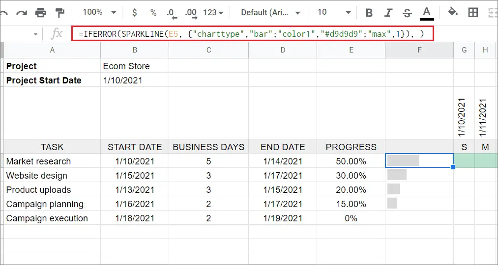
Notice that the light gray bar indicates the progress of each task. The higher the % value, the longer the gray progress bar.
That’s all about creating a Gantt chart in Google Sheets using conditional formatting rules.
How To Export Google Sheets Gantt Chart To Excel
If you have created a Gantt chart in Google Sheets, you can easily export it to Microsoft Excel with a few simple steps.
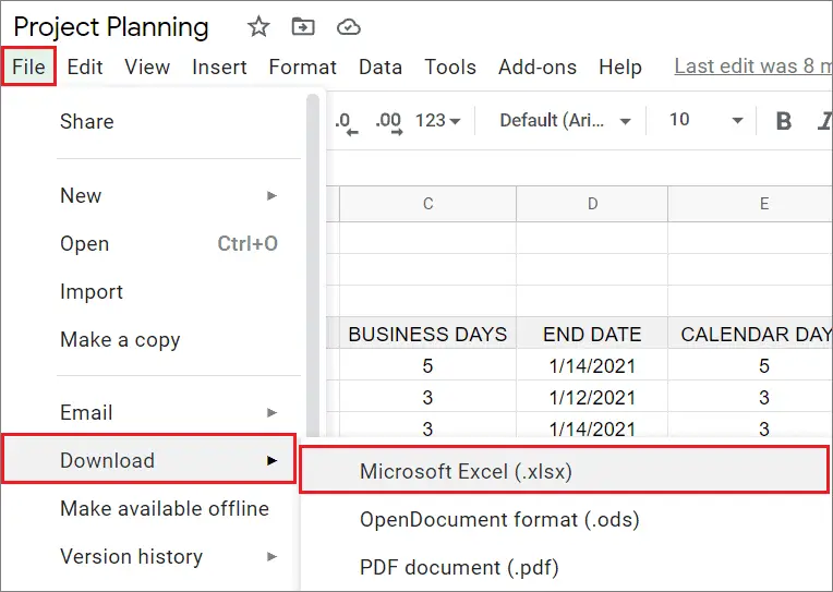
To begin with, click on the File tab and choose Download from the drop-down menu. Next, choose Download and select Microsoft Excel from the nested menu.
You can open this simple project timeline file in Excel format post the download process. That’s all about how to create a Gantt chart in Google Sheets.
Conclusion
A Google Gantt chart is a handy tool for Google Sheets project management and planning. You can use it to create tasks and allocate resources to ensure your project comes to fruition over a particular time constraint. Beginners can use a Google sheet to create a with creating a simple Gantt chart in Google Sheets to get the hang of managing projects.
Apart from a ready-made Gantt chart template, you can also opt for project planning tools to manage your projects. There are two simple ways to create a Google Sheets Gantt chart. Users can opt for any method as per their choice. You can also use an Excel spreadsheet to create a Gantt chart.
FAQs
Where can I make a Gantt chart?
You use Google Sheets or project planning and management software to make a Gantt chart.
How do I make a Gantt chart in Google Sheets?
You can make a Gantt chart using conditional formatting rules or using a stacked bar chart in Google Sheets.
Can we make a Gantt chart in Google doc or Google slide?
You can make a Gantt chart in Google Slides, but it’s not possible to make one in Google Docs.


