Slicing and dicing is an important aspect when it comes to analyzing data in Microsoft Excel and Google Sheets. Sorting and filtering are two important features offered by these tools for extracting specific data from a gigantic dataset. Hence, users need to know how to use filter function in Google Sheets.
In comparison to the filter feature, the filter function is more dynamic. If you make changes to your source data and cell references, the filtered view will also change accordingly. This factor makes the filter function a great choice to work with while creating dashboards or reports. Apart from the filter function, you can also use conditional formatting in Google Sheets to identify relevant chunks of data in a large dataset.
How To Use Filter Function In Google Sheets To Obtain Specific Data
The filter function allows users to filter a dataset based on various conditions. Let’s take a glance at the different scenarios in which we can use this function to filter and obtain specific data.
FILTER Function Syntax
Before we move on to the main process of usage, it’s essential to know how to represent the Google Sheets filter function in the right manner.
=FILTER(range, condition 1, [condition 2...,])range – The data range of cells on which you wish to apply the filter function.
condition 1 – It is an array, row, or column similar in length or width to the corresponding row or column of the range. It contains evaluated TRUE or FALSE values.
condition 2 – Optional or additional array similar to condition 1 in terms of the format.
You cannot use the row and column conditions in the same function. The filter criteria has to be either of the row type or the column type.
Filter Data Based On Single Condition
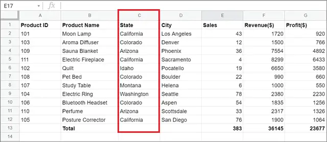
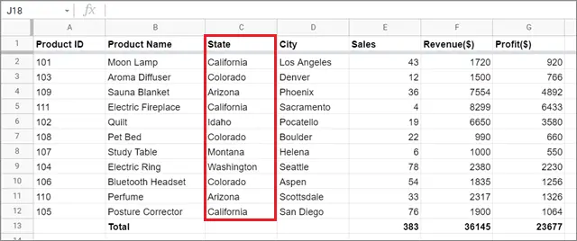
First, let’s begin with the basics with the simple function of the filter formula in cell. Let’s say you want to filter the sales data from California in this Google sheet given below. Now that we have established the additional conditions, it’s time to apply the filter function in Google Sheets.
In this example, we will be working on the range of values from column C in the dataset.
The Google Sheets formula for the given filter condition and range reference will be as given below.
=FILTER(A2:G12,C2:C12,“California”)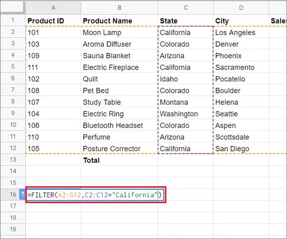
Once you enter the formula, hit the Enter key to see the filtered result in the selected cell.
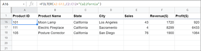
In this case, A2:G12 is the entire data range that we are working upon. C2:C12=“California” tells Google Sheets to check the column cells from C2 to C12 for the word ‘California’ and filter the data accordingly.
Note: The filter function is a dynamic array, i.e, it returns values over adjacent cells. While calculating the filtered result, make sure you have enough blank cell count for the result to fit in. For instance, if you need five cells horizontally to display a result and one of those cells is filled, the Google Sheets filter function will show a #REF error. So, make sure you count cells properly before executing the function.
Google Sheets will also give you the reason for that error, citing the filled cell as the cause of the issue. Once you delete the content in the filled cell, the filter function will automatically return the result.
The grey line under the column header indicates that the header row has been frozen for better convenience. You can freeze the header row if you are executing the filtered results right below the main data, as we have done in this example.
Filter Data For Multiple Conditions Using AND Function
We have seen how the filter function in Google Sheets works with a single condition. Now, let’s try out multiple criteria and additional functions.
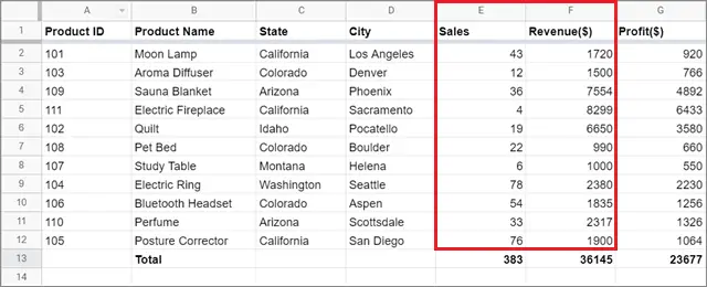
In the given Sales Sheet, you have to filter the states which have brought in more than 20 sales and amassed a revenue greater than $2000. So, here we will be working with columns E and F respectively.
To start with, select the cell and enter the entire formula in the cell based on the condition. The formula will be as given below.
=FILTER(A2:G12,E2:E12>20,F2:F12>2000)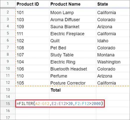
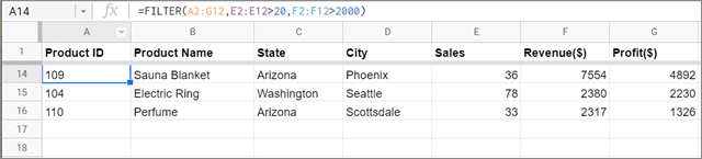
Next, hit the Enter key to calculate the result. You can see that the Google Sheets filter function has successfully returned values that adhere to the conditions mentioned above.
You can also combine more than two conditions in the same filter function and obtain the result. The filter function is a good alternative for those who aren’t well-versed in creating pivot tables in Google Sheets.
Filter Data On Multiple Conditions Using OR
Previously, we saw how to use the filter function in Google Sheets using the AND function. Now, let’s look at the opposite.
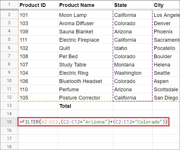
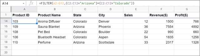
In this case, we have to extract data from either Arizona or Colorado. So, we need to work with two conditions on a single column, i.e., entries in column C.
Select the cell and enter the single formula to solve the query as shown below. The OR operation is represented by the ‘+’ sign in the function.
=FILTER(A2:G12,(C2:C12=“Arizona”)+(C2:C12=“Colorado”))Here, the brackets on each side of the ‘+’ sign represent the conditions used with the OR function.
Press the Enter key to get the unique values of the filtered result.
The OR operator checks the selected array of multiple rows for the defined conditions. If the condition matches the requirement, it is a TRUE condition and is assigned a ‘1’ value. Similarly, the FALSE condition is assigned a ‘0’ value and the filter function doesn’t include it in the result. Users can also use mixed conditions in the OR function to get the filtered result.
Filter Top Results
Sometimes, when the dataset is very long, beginners can have a tough time finding out the best records in the data. In this example, we will see how to use the filter function in Google Sheets to find out the top results in a dataset.
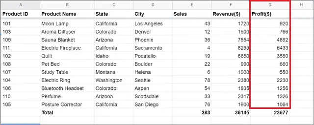
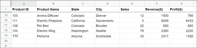
In this scenario, the condition is to find the top five products from the list of products stated in column B that have got the highest profits irrespective of the country names. So, here we will work on column G.
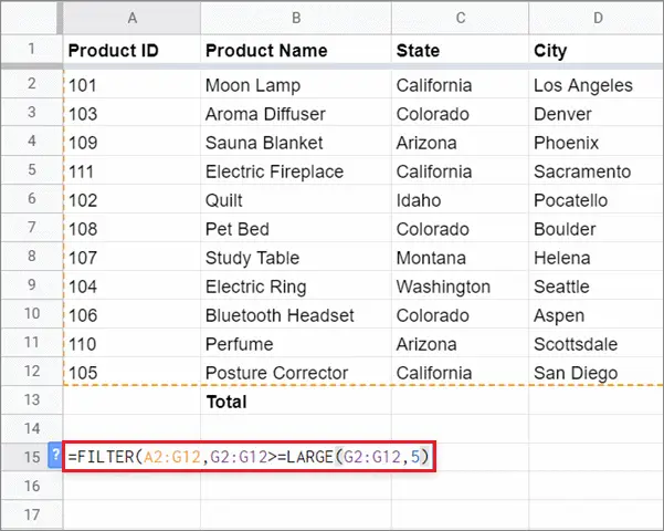
To begin with, enter the Google Sheets filter formula as per the conditions you wish to satisfy. In our case, the formula will be as given below.
=FILTER(A2:G12,G2:G12>=LARGE(G2:G12,5)When it comes to finding the top results in a datasheet, you need to use the nested LARGE function in the filter formula.
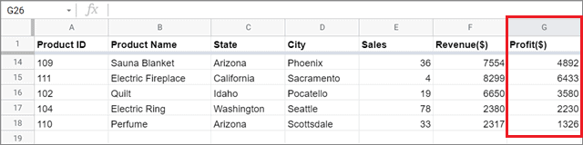
Now, press the Enter key to get the filtered result. You can see which five products have topped the sales figures.
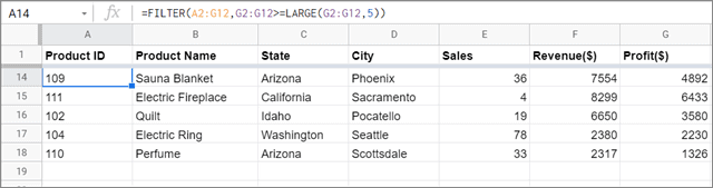
The LARGE function in the formula extracts the defined value and then compares the remaining values in the data range to find out the top records. Here, we asked Google Sheets to find the fifth highest value and then compare it with all other records in the selected cell range.
The Google Sheets filter formula will return the fifth highest value and all other greater values to satisfy the given criteria.
In case you want to find the bottom values, you can use the SMALL function instead of the LARGE function, as shown below.
=FILTER(A2:G12,G2:G12<=SMALL(G2:G12,5)This formula will give you the bottom five records.
Use Filter Function In Google Sheets To Sort The Top Results
Notice that in the previous section, we successfully extracted the top five records from the dataset using the filter function in Google Sheets. However, the obtained result isn’t displayed in the perfect ascending order.
In this case, we need to use a nested filter function in the sort function to arrange the data from highest to lowest value. Here, we will be working with column G.
Enter the sort function with the nested filter function in a cell. Select the cell in which you entered the filter function and add the sort function to it using the formula bar.
=SORT(FILTER(A2:G12,G2:G12>=LARGE(G2:G12,5)),7,FALSE)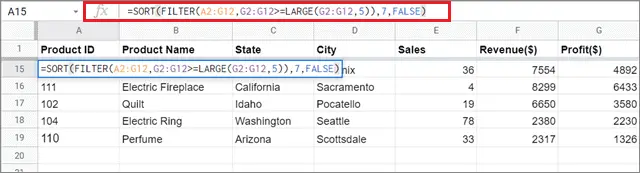
Then, hit the Enter key to obtain the result. You can see that the data in the column has been arranged from the highest to the lowest value.
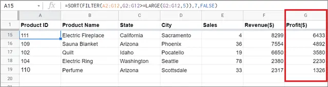
In the sort function, the number ‘7’ denotes the column number of the column in which you need to arrange the data. The FALSE value tells Google Sheets to arrange the data in descending order from highest to lowest. If you want it in ascending order, you can leave the argument blank or enter TRUE.
Filter Odd Or Even Records
Sometimes, you may receive unstructured data from your peers; the records may be placed in alternate rows in a sheet. In this case, you can regroup the data properly by filtering the odd or even rows, depending on how the records are placed.
You can also modify the data and instruct Sheets to filter every third, fourth, fifth, or nth row. In the current scenario, let’s take a look at how to use the filter function in Google Sheets to filter even records in the sales sheet we have used for the previous ways.
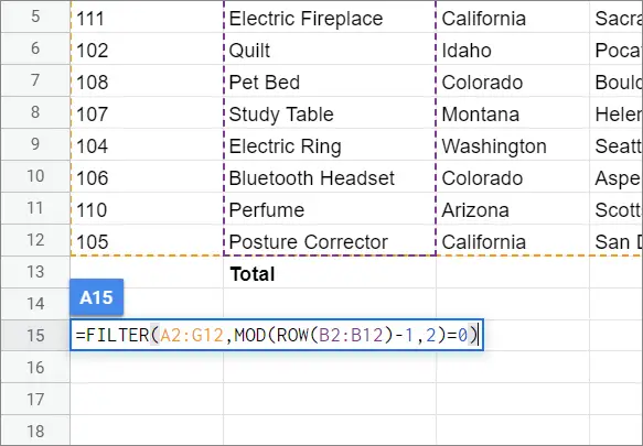
Enter the formula for filtering odd or even records as per your choice. Here, we have chosen to filter the even rows and entered the formula accordingly.
=FILTER(A2:G12,MOD(ROW(B2:B12)-1,2)=0)The main point to remember here is the role of the ROW function. The ROW function considers all the rows in the selected dataset. We subtract 1 from the ROW function because the selected dataset starts from the second row of the Google spreadsheet.
The number ‘2’ denotes the fact that we are filtering every second row as even and odd numbers are always alternate. If you want to filter every third row, you can write ‘3’ instead.
Once you enter the Google Sheets filter function for filtering data, hit the Enter key to get the result. You will see all the even records have been filtered successfully out of the selected dataset.
If you want to select odd number records from the dataset, just enter the formula given below.
=FILTER(A2:G12,MOD(ROW(B2:B12)-1,2)=1)The only change in the even and odd equation is the difference between 0 and 1 at the end of the formula.
That’s all about how to use the Google Sheets filter formula on multiple sheets. For better summarization of data, you can also use the VLOOKUP in Google Sheets. Further, if you want to create a drop-down list in your datasheet, you can use data validation for this purpose.
Conclusion
The filter function is a highly useful tool that allows Google Sheets users to summarize data in large datasets. You can use the filter function in Google Sheets under various circumstances to obtain different types of results. The filter function can also be used on the Google Sheets mobile app; you need to follow the same steps as you did for executing the function on the PC.
Make sure you don’t get confused between the filter feature and the filter function. The basic filter feature can filter data based on one condition at a time; you can execute it using the built-in filter icon in the toolbar. The filter function offers better flexibility as it allows users to filter data based on multiple columns and conditions using complex mathematical equations.


